Electronic Warfare and Radar Systems Engineering Handbook |
|
|
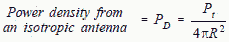
POWER DENSITY Radio Frequency (RF) propagation is defined as the travel of electromagnetic waves through or along a medium. For RF propagation between approximately 100 MHz and 10 GHz, radio waves travel very much as they do in free space and travel in a direct line of sight. There is a very slight difference in the dielectric constants of space and air. The dielectric constant of space is one. The dielectric constant of air at sea level is 1.000536. In all but the highest precision calculations, the slight difference is neglected. From chapter 3, Antennas, an isotropic radiator is a theoretical, lossless, omnidirectional (spherical) antenna. That is, it radiates uniformly in all directions. The power of a transmitter that is radiated from an isotropic antenna will have a uniform power density (power per unit area) in all directions. The power density at any distance from an isotropic antenna is simply the transmitter power divided by the surface area of a sphere (4πR2) at that distance. The surface area of the sphere increases by the square of the radius, therefore the power density, PD, (watts/square meter) decreases by the square of the radius. [1]
Pt is either peak or average power depending on how PD is to be specified. Radars use directional antennas to channel most of the radiated power in a particular direction. The Gain (G) of an antenna is the ratio of power radiated in the desired direction as compared to the power radiated from an isotropic antenna, or:
The power density at a distant point from a radar with an antenna gain of Gt is the power density from an isotropic antenna multiplied by the radar antenna gain. Power density from radar, Pt is either peak or average power depending on how PD is to be specified. Another commonly used term is effective radiated power (ERP), and is defined as: ERP = Pt Gt A receiving antenna captures a portion of this power determined by it's effective capture Area (Ae). The received power available at the antenna terminals is the power density times the effective capture area (Ae) of the receiving antenna.
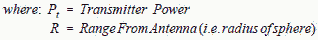
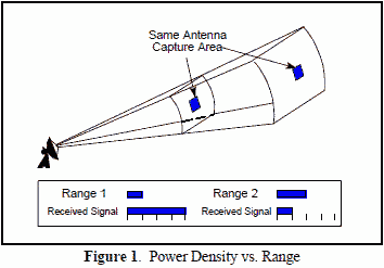
For a given receiver antenna size the capture area is constant no matter how far it is from the transmitter, as illustrated in Figure 1. Also notice from Figure 1 that the received signal power decreases by 1/4 (6 dB) as the distance doubles. This is due to the R2 term in the denominator of equation [2].
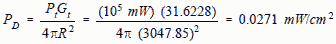
Sample Power Density Calculation - Far Field (Refer to Section 3-5 for the definition of near field and far field) Calculate the power density at 100 feet for 100 watts transmitted through an antenna with a gain of 10. Given: Pt = 100 watts Gt = 10 (dimensionless ratio) R = 100 ft This equation produces power density in watts per square range unit.
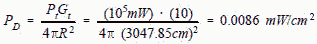
For safety (radiation hazard) and EMI calculations, power density is usually expressed in milliwatts per square cm. That's nothing more than converting the power and range to the proper units. 100 watts = 1 x 10² watts = 1 x 10⁵ mW 100 feet = 30.4785 meters = 3047.85 cm.
However, antenna gain is almost always given in dB, not as a ratio. It's then often easier to express ERP in dBm.
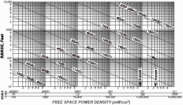
ERP (dBm) = Pt (dBm) + Gt (dB) = 50 + 10 = 60 dBm To reduce calculations, the graph in Figure 2 can be used. It gives ERP in dBm, range in feet and power density in mW/cm2. Follow the scale A line for an ERP of 60 dBm to the point where it intersects the 100 foot range scale. Read the power density directly from the A-scale x-axis as 0.0086 mW/cm2 (confirming our earlier calculations).
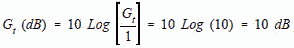
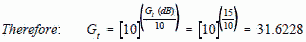
Figure 2. Power Density vs Range and ERP Example 2 When antenna gain and power (or ERP) are given in dB and dBm, it's necessary to convert back to ratios in order to perform the calculation given in equation [2]. Use the same values as in example 1 except for antenna gain. Suppose the antenna gain is given as 15 dB: Gt (dB) = 10 Log (Gt)
Follow the 65 dBm (extrapolated) ERP line and verify this result on the A-scale X-axis. Example 3 - Sample Real Life Problem
Given the following:
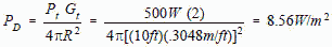
Jammer power: 500 W (Pt = 500) Jammer line loss and antenna gain: 3 dB (Gt = 2) Missile antenna diameter: 10 in Missile antenna gain: Unknown Missile limiter protection (maximum antenna power input): 20 dBm (100mW) average and peak. The power density at the missile antenna caused by the jammer is computed as follows:
The maximum input power actually received by the missile is either: Pr = PD Ae (if effective antenna area is known) or Pr = PD Gmλ / 4π (if missile antenna gain is known) To cover the case where the missile antenna gain is not known, first assume an aperture efficiency of 0.7 for the missile antenna (typical). Then: Pr = PD Aη = 8.56 W/m2 (π)[ (10/2 in)(.0254 m/in)]2 (0.7) = 0.3 watts Depending upon missile antenna efficiency, we can see that the power received will be about 3 times the maximum allowable and that either better limiter circuitry may be required in the missile or a new location is needed for the missile or jammer. Of course if the antenna efficiency is 0.23 or less, then the power will not damage the missile's receiver. If the missile gain were known to be 25 dB, then a more accurate calculation could be performed. Using the given gain of the missile (25 dB= numeric gain of 316), and assuming operation at 10 GHz (λ = .03m) Pr = PD Gmλ2 / 4π = 8.56 W/m (316)(.03) / 4π = .19 watts (still double the allowable tolerance
Table of Contents for Electronics Warfare and Radar Engineering Handbook Introduction | Abbreviations | Decibel | Duty Cycle | Doppler Shift | Radar Horizon / Line of Sight | Propagation Time / Resolution | Modulation | Transforms / Wavelets | Antenna Introduction / Basics | Polarization | Radiation Patterns | Frequency / Phase Effects of Antennas | Antenna Near Field | Radiation Hazards | Power Density | One-Way Radar Equation / RF Propagation | Two-Way Radar Equation (Monostatic) | Alternate Two-Way Radar Equation | Two-Way Radar Equation (Bistatic) | Jamming to Signal (J/S) Ratio - Constant Power [Saturated] Jamming | Support Jamming | Radar Cross Section (RCS) | Emission Control (EMCON) | RF Atmospheric Absorption / Ducting | Receiver Sensitivity / Noise | Receiver Types and Characteristics | General Radar Display Types | IFF - Identification - Friend or Foe | Receiver Tests | Signal Sorting Methods and Direction Finding | Voltage Standing Wave Ratio (VSWR) / Reflection Coefficient / Return Loss / Mismatch Loss | Microwave Coaxial Connectors | Power Dividers/Combiner and Directional Couplers | Attenuators / Filters / DC Blocks | Terminations / Dummy Loads | Circulators and Diplexers | Mixers and Frequency Discriminators | Detectors | Microwave Measurements | Microwave Waveguides and Coaxial Cable | Electro-Optics | Laser Safety | Mach Number and Airspeed vs. Altitude Mach Number | EMP/ Aircraft Dimensions | Data Busses | RS-232 Interface | RS-422 Balanced Voltage Interface | RS-485 Interface | IEEE-488 Interface Bus (HP-IB/GP-IB) | MIL-STD-1553 & 1773 Data Bus | This HTML version may be printed but not reproduced on websites. |
|

 [2]
[2] 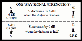
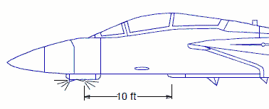 Assume we are trying to determine if a jammer will damage the circuitry of a missile
carried onboard an aircraft and we cannot perform an actual measurement. Refer to the diagram at the right.
Assume we are trying to determine if a jammer will damage the circuitry of a missile
carried onboard an aircraft and we cannot perform an actual measurement. Refer to the diagram at the right.