|
January 1944 Electronics
") [Table of Contents] [Table of Contents]
Wax nostalgic about and learn from the history of early electronics.
See articles from Electronics,
published 1930 - 1988. All copyrights hereby acknowledged.
|
Here is the follow-up article
from
Phillip H. Smith's original "Transmission
Line Calculator" of his Smith Chart in the January 1939 issue of Electronics
magazine. "An Improved Transmission Line Calculator" appeared in the January 1944 issue. Mr. Smith worked at the Radio
Development Department of Bell Telephone Laboratories in New York City. He states
in part, "The calculator is, fundamentally, a special kind of impedance coordinate
system, mechanically arranged with respect to a set of movable scales to portray
the relationship of impedance at any point along a uniform open wire or coaxial
transmission line to the impedance at any other point and to the several other electrical
parameters. These other parameters are plotted as scales along the radial arm and
around the rim of the calculator, both of which are arranged to be independently
adjustable with respect to the main impedance coordinates." A thorough discussion
of the Smith chart's constructions and examples of its use are presented.
An extension of the "calculator" originally published in ELECTRONICS
in January 1939. New parameters have been added and accuracy has been improved
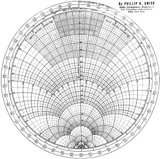
Fig. 1 - Circular transmission line calculator with separately
rotatable "wavelengths" scale around rim. Transparent arm shown in Fig. 2 is
pivoted at the center of the calculator. Slider is slipped on arm as crosshair indicating
mechanism.
By Phillip H. Smith
Radio Development Department
Bell Telephone Laboratories, New York City
There was developed and has been in use in the Bell Telephone Laboratories for
a number of years a particularly useful form of calculator for solving radio transmission
line problems. The calculator was originally described in ELECTRONICS* where it
was presented in "cut-out" form. The impetus given to radio development by the war
has promoted considerable interest in this calculator among engineers and research
workers, particularly in the field of u-h-f technique where electrical measurements
must be made indirectly. Accordingly, it has been felt desirable to again present
at this time a comprehensive description of the device. Several new and useful parameters
have been added to the original design and the entire calculator has been redrawn
to improve its accuracy and facilitate reading the coordinates.
The calculator is, fundamentally, a special kind of impedance coordinate system,
mechanically arranged with respect to a set of movable scales to portray the relationship
of impedance at any point along a uniform open wire or coaxial transmission line
to the impedance at any other point and to the several other electrical parameters.
These other parameters are plotted as scales along the radial arm and around the
rim of the calculator, both of which are arranged to be independently adjustable
with respect to the main impedance coordinates. All of the parameters are related
to one another and specific solutions to a given problem are obtainable through
the use of an adjustable cross-hair index along the radial arm, which extends to
intersect the scales around the rim. The parameters which are plotted on the calculator
include:
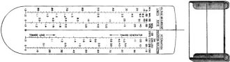
Fig. 2 - Transparent arm shown is pivoted at the center
of the calculator in Fig. 1. Slider is slipped on arm as crosshair indicating
mechanism. Fig. 1 and Fig. 2 are at the same scale for printing.
I. Impedance, or admittance, at any point along the line. (a) Reflection coefficient
magnitude. (b) Reflection coefficient angle in degrees.
II. Length of line between any two points in wavelengths.
III. Attenuation between any two points in decibels. (a) Standing wave loss coefficient.
(b) Reflection loss in decibels.
IV. Voltage or current standing wave ratio. (a) Standing wave ratio in decibels.
(b) Limits of voltage and current due to standing waves.
A brief discussion of each of the several parameters and the manner in which
they may be evaluated from the calculator will be given. The impedance at any point
along a transmission line is, unless otherwise defined, normally considered to be
that impedance which would be measured if the line were cut at that point and measurements
were made looking into the line section which is connected to the load.
Impedance - General Considerations
The impedance at any point along the line and the power reaching this point from
the generator completely determine the magnitude of the current and voltage and
their phase relationship at that point. For a steady state, the generator impedance
itself, as well as the impedance looking towards the generator from any point along
the line where it may have been considered to have been cut, can in no way affect
the distribution of current or voltage along the transmission line to which the
generator is connected.
In other words, the generator impedance can have no effect upon the standing
wave position or amplitude ratio or upon the relation of the standing wave to the
impedance distribution (locus of impedances) along the line. The generator impedance
can affect only the power delivered to the transmission line and consequently the
amplitude of the current or voltage all along the line, proportionately. The calculator
relates the series components of the impedances thus considered at any point along
a transmission line to a number of other parameters which will be discussed individually.
Impedance Coordinates - Central of Calculator Area
The series impedance components are represented on the calculator as two orthogonal
families of circular curves plotted upon the central circular disc, one family of
curves representing resistances and the other reactances. All impedances, both known
and unknown, are read thereupon. To make the calculator of general application,
these impedance coordinates are labeled as a fractional part of the characteristic
impedance of the line (a fixed parameter in any given problem which may be evaluated
from the physical dimensions of the line.)**
It is therefore necessary when using the calculator for solving problems involving
the impedance at any point to first divide the components of all known impedances
by the characteristic impedance of the line, then obtain a solution from the calculator
which, if an impedance, will be expressed as a fraction of the characteristic impedance
of the line, and finally to multiply this solution by the characteristic impedance
to obtain the answer in ohms. The characteristic impedance is usually a "real" number,
i.e., a pure resistance, for radio transmission lines, which makes this procedure
a relatively simple one.
The relation between the impedance of the line at any point and the other parameters
listed above is evaluated with the aid of the cross-hair index line on the radial
arm as described later.
Equivalent Parallel Components of Impedance
The calculator also provides a means for converting the series components of
impedances to their equivalent parallel resistance and parallel reactance components.
This is accomplished by setting the series components under the cross-hair index
line on the radial arm and then moving the latter to the diametrically opposite
point on the calculator and taking the reciprocal of the values read at that point
as the equivalent parallel resistance and parallel reactance. (A reciprocal scale
is provided along the radial arm.) The equivalent parallel component of resistance
is useful in problems where it is desired to evaluate the magnitude of the voltage
and to avoid converting the problem to one involving admittances.
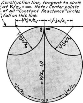
Fig. 3 - Construction of admittance circles.
Admittance Coordinates
The calculator relates the series components of admittances, as well as impedances,
to the various other parameters listed above and accordingly the coordinates may
be considered to be admittance coordinates if preferred. In this case the coordinate
axis (real) labeled "Resistance Component (R/Z0)" becomes the Conductance
Component (a/Yo) axis, the scale units then indicating a fractional part
of the characteristic admittance of the line. Likewise, the coordinate axis (imaginary)
labeled "Positive Reactance Component (+jX/Z0)" becomes the Positive
Susceptance Component (+jb/Y) axis and in the negative direction the Negative Susceptance
Component (-jb/Y). Admittance is defined as Y = a + jb and it is important to remember
that capacitance is considered to be a positive susceptance and inductance a negative
susceptance. The direction of rotation indicated on the calculator in moving from
one point to another is the same whether impedance or admittance coordinates are
considered.
Fig - Construction of "constant reactance" curves ±jx/Z0
Converting Impedances to Admittances
Impedances may be converted to admittances, or vice versa, by going to a diametrically
opposite point on the calculator, as described above for obtaining the equivalent
parallel resistance components, and reading the values at that point as conductance
and susceptance.
Reflection Coefficient
The impedance (or admittance) at any point along a uniform transmission line
is completely defined by the amplitude and phase angle of the "reflection coefficient"
at that point. It is often convenient to think of transmission line phenomena in
terms of the magnitude and phase relationship of reflected and incident traveling
waves, i.e., the reflection coefficient of the transmission line under consideration.
The magnitude of the reflection coefficient is expressed by a number between
0 and 1.0, which represents the ratio of reflected to incident voltage at the point
under consideration. If the attenuation of the line is negligible the magnitude
of the reflection coefficient will be a constant at all points along the line for
a given load impedance resulting in a given standing wave amplitude ratio along
the line.
The magnitude of the reflection coefficient is plotted as a scale along the radial
arm. The phase angle of the reflection coefficient is directly related to the impedance
and accordingly is indicated on the calculator as a scale around the rim of the
impedance coordinate system.
All impedances radially in line have a constant reflection coefficient phase
angle. This phase angle is the angle by which the reflected wave lags the incident
wave at the point along the line under consideration. Where these two waves add
in phase to give a maximum voltage the impedance is resistive and greater than the
characteristic impedance of the line, and the angle of the reflection coefficient
is zero degrees. Going towards the generator from this point, the departure from
zero phase angle is linearly related to the distance traversed. The reflected voltage
wave at first lags the incident voltage wave (having the longer path to traverse)
and the phase angle of the reflection coefficient is considered to be negative for
the first quarter wavelength from the voltage maximum point in the direction of
the generator. The reactive component of the impedance in this region is negative.
At the exact quarter-wavelength (90 deg.) point the incident and reflected voltage
waves are exactly out of phase and the angle of the reflection coefficient is ±180
deg. Continuing in the same direction towards the generator, the two waves become
increasingly more in-phase and in this region between one-quarter and one-half wavelength
from the voltage maximum point towards the generator, where the reactive component
of the impedance is inductive, the reflected wave leads the incident wave and the
reflection coefficient has a positive angle. The relationship between the magnitude
of the reflection coefficient and the standing wave amplitude ratio may be derived
fronts the fact that at the voltage maximum point the incident and reflected waves
add in phase, whereas, at the voltage minimum point they are exactly out of phase,
thus
k = magnitude of the voltage reflection coefficient
VR = reflected voltage
VI = incident voltage
Length of Line-Movable Distance Scale Around Rim
Impedances along a uniform transmission line vary cyclically, repeating every
half wavelength if the line has negligible attenuation. Thus, for any given termination
the impedance locus path in going along the line in either direction from any initial
starting point will close upon itself in exactly one-half wavelength effective length.
The circular calculator is arranged so that one trip around the impedance coordinated
disc at any constant distance from the center corresponds to a movement of just
one-half wavelength along the transmission line. The length scale around the rim
of the calculator is linear and its zero position may be adjusted so that measurements
can be started from a point radially in line with any known impedance point on the
coordinates and carried in either direction, i.e., either "towards the generator"
or "towards the load" to a point where it may be desired to know the impedance.
Uniform transmission lines with air dielectric and negligible attenuation have
an "effective length" equivalent to the length of the wave in free space and no
correction is required for the length scale. However, any solid dielectric material
in the field of the conductors causes a reduction in the length of the standing
wave which is proportional to 1/√K
where K is the dielectric constant. This applies to lines where the entire field
is confined to a homogeneous dielectric such as rubber-insulated coaxial lines.
In coaxial lines, for example, where bead insulators are used, if the beads are
spaced closer than about 1/36th wavelength, the line may be considered to have a
uniform effective dielectric constant. The length scale refers to the "effective
length" of the line.
As further discussed in the section entitled "Standing Wave Ratio," the relation
between impedance and current distribution (standing waves), especially with respect
to their position along the line, is often conveniently referred to the pure resistance
points and length measurements are often made with reference to one end or the other
of the "real" axis, at which points the maximum and minimum current and voltage
points occur.
Construction of "constant resistance" curves R/Z0
Any line length in excess of one-half wavelength can be reduced to an equivalent
shorter length to bring it within the scale range of the calculator by subtracting
the largest possible whole numbers of half wavelengths therefrom.
Construction of "constant resistance" curves R/Z0
.
Scales Along Radial Arm
A number of the parameters are uniquely related to one another as well as to
the magnitude of the reflection coefficient previously described. These parameters
are conveniently plotted as scales along the radial arm in nomograph form. Their
relationship may be evaluated through the use of the sliding index line which permits
reading any or all of the several scales at the intersection of the slider index
line. A given set of such values are also related to a given impedance locus which
is traversed upon the impedance coordinates at the cross index line intersection
when the radial arm is rotated once around the calculator. The several related parameters
plotted along the radial arm in nomograph form include the following:
(1) Attenuation in 1-db steps (due to loss resistance of line, leakage, and dielectric
loss).
(2) Standing wave loss coefficient (due to increased average current and voltage).
(3) Reflection loss (or gain) in decibels.
(4) Reflection coefficient magnitude (voltage).
(5) Standing wave ratio (SWR) of maximum to minimum current or voltage.
(6) Standing wave ratio expressed in decibels (20 log10SWR) .
(7) Relative voltage or current at maximum and minimum points for constant power.
Attenuation
Attenuation causes the impedance locus along a uniform transmission line to spiral
inward toward the center of the calculator from the initial starting point when
going from the load end of the line "toward the generator", and to spiral outward
toward the rim when going from an initial starting point "toward the load". The
rate at which this spiral locus approaches the center (or the rim) depends directly
upon the attenuation per unit length of line as well as upon the initial starting
point.
Impedances near the rim (encountered along a line bearing a large standing wave)
are altered to a greater extent by a db unit of attenuation, for example, than impedances
near the center. The attenuation scale is conveniently plotted along the radial
arm since it is a measure of the rate at which the impedance locus spirals in or
out.
The starting point for this nonlinear scale must be capable of being set at any
impedance point on the coordinates. Also, the scale must be capable of measuring
attenuation in either direction from the starting point depending upon whether conditions
are to be observed in a direction from an initial starting point "toward the load"
or "toward the generator". To accomplish this the scale is laid out without markings,
in 1-db steps. Thus, to take into account an attenuation of say 3 db it is necessary
to count off three 1-db intervals in the proper direction along the attenuation
scale from whatever starting point may have existed, before reading the answer on
the impedance coordinates. The proper direction to go in correcting the impedance
for attenuation of the line is indicated upon the attenuation scale itself.
Standing Wave Loss Coefficient
The scale along the radial arm labeled "S.W. Loss Coef." shows the additional
copper or dielectric loss due to the presence of standing waves in the vicinity
of the standing wave measurement. This added loss coefficient, which multiplies
the calculated loss in decibels for a matched line, does not affect the line impedance.
This added dissipation within the line is caused by the fact that the line conducts
more average current and is required to withstand more average voltage for a given
transmitted power when standing waves are present than would normally be the case
if the line were properly matched.
Since copper losses at any point are proportional to the square of the current
and dielectric losses or leakage losses are proportional to the square of the voltage,
the percentage increment in losses applies equally to either type of loss. This
loss coefficient refers more accurately to the increase in losses over a half wavelength
of transmission line in the immediate vicinity of the standing wave measurement.
In cases where the copper and dielectric or leakage losses are approximately equal
it holds closely for any fractional part of a half wavelength. In this special case,
when moving along the line, the change in copper loss due to the standing current
wave is approximately compensated by an equal and opposite change in dielectric
or leakage due to the reversed slope of the voltage wave, resulting in a substantially
uniform increase in loss for any fractional part of a half wavelength. If, due to
attenuation, the standing wave ratio and consequently the standing wave loss coefficient
change in moving along the line, for example several wavelengths, then the increased
loss for the entire line section traversed lies between the coefficient limits indicated
at each end.
Reflection Loss (or Gain)
The "reflection loss" may be derived from the reflection coefficient (k), which
as described is the ratio of reflected to incident voltage. The reflection loss
in decibels is
db = log10 10 (Pabsorbed / Pincident
) (3)
The absorbed power is proportional to the square of the incident voltage (VI2)
minus the square of the reflected voltage (VR)2 and the incident
power is proportional to the square of the incident voltage (VI2).
Therefore
db = 10 log10 (VI2 -
VR2)/VI2
(4)
= 10 log10 1 - (VR/VI)2
(5)
= 10 log10 (1 - k2)
(6)
If the attenuation of the line is negligible, the "reflection loss" does not
represent an actual loss of power, for if an impedance match is made at the sending
end of the transmission line with the generator, a "reflection gain" takes place
which neutralizes the "loss" at the load end. When the attenuation is not negligible,
the reflection loss at the input (which actually represents an equivalent reflection
gain when the input impedance to the line is matched to the generator impedance)
will be less than the reflection loss at the load. This difference between the reflection
loss, which can be read on the radial arm of the calculator, at the two ends of
the line represents an additional dissipation loss within the line itself which
is caused by the increased average current and voltage.
Standing Wave Ratio
The standing wave ratio (SWR) is expressed as a number greater than 1.0. The
position of the standing wave along the line is significant and it is important
to remember in using the calculator that it is always at a current maximum point
that the impedance is a minimum and "real", i.e., the current maximum point always
falls along the R/Z0 axis (when Z0 is real) at a point between
0 and 1.0.
Likewise, it is important to remember that the current minimum point always falls
along the R/Z0 axis at a point between 1.0 and ∞. The voltage standing
wave is always positioned just a quarter wavelength along the line either side of
the position of the current standing wave, so that a voltage minimum point on the
wave will always coincide in position with a current maximum point and likewise
a voltage maximum point will always coincide in position with a current minimum
point.
Thus, the relative position between impedance and current distribution (standing
waves) is most conveniently referred to these pure resistances or real impedance
positions along the R/Z0 axis, and standing wave measurements are made
with respect to these points along the line.
A given standing wave ratio uniquely defines the locus of impedances encountered
along a uniform transmission line when the latter has negligible attenuation. To
determine this locus the slider along the radial arm is set to coincide with the
known standing wave ratio. The impedance locus then appears at the intersection
of the cross-hair index when the arm is swung around through one complete revolution.
The passage of this intersection point once around the calculator is equivalent
to moving one-half wavelength along the transmission line, and it is thus seen that
the impedance circle locus closes upon itself and then repeats for any two points
a half wavelength apart and greater. The impedance locus passes through the resistance
axis twice in one revolution of the arm about the coordinates, at which two positions
the impedance is maximum and minimum respectively and, as described, the current
and voltage, likewise, go through maximum and minimum values.
The measurement of standing waves is often accomplished through the use of sliding
capacitive or inductive probes (depending upon whether voltage or current waves
respectively are to be observed). The output power taken from the probe is at a
low level compared to that flowing in the main line so as not to disturb the line
characteristics.
Standing Wave Ratio Expressed in dB
The probe output is amplified through a double detection receiver. The receiver
includes an attenuator in its i-f amplifier circuits which is calibrated in decibels.
The rectified output of the receiver is indicated on a reference level meter. It
is convenient to adjust the meter output to an arbitrary reference mark and observe
the change in attenuation required when going from a maximum to a minimum point
along the standing wave. The standing wave amplitude ratio may then be expressed
in decibels. Thus, a 6-db standing wave will have a ratio of maximum to minimum
amplitude of 2 to 1. Used in this sense the term has no significance insofar as
loss or power ratio is concerned. A scale is provided to permit expressing the standing
wave ratio in decibels.
Relative Voltage or Current at Maximum and Minimum Points
If a transmission line is conducting a given amount of power it will do so most
efficiently when standing waves are eliminated. However, there are cases when it
will be acceptable or even desirable to permit standing waves to exist. In this
case the line must be designed to withstand the increase in current and in voltage
at the antinodes. This increase at the antinodes in both current and voltage (and
decrease at the nodes) is plotted along the radial arm and refers to the increase
or decrease at these points over what it would be if the line were properly terminated
and were conducting the same amount of power to the load.
The voltage magnitude (E) at any point along the line in terms of the equivalent
parallel resistance (Rpar) component and the power (P) is
E = √(Rpar x P)
(7)
whereas the current magnitude (I) at any point in terms of the series resistance
(Rser) component and the power (P) is
 (8)
(8)
In either case, the reactive component is not involved.
At the maximum and minimum impedance points the series and parallel components
become the same. At these points the maximum and minimum current and voltage are
conveniently evaluated from the standing wave ratio, characteristic impedance, and
power as follows:
where Z0 = characteristic impedance in ohms.
P = power in watts.
SWR = voltage or current standing wave ratio expressed as a number greater than
unity.
Example for Use of the Calculator
A coaxial r -f transmission line having a characteristic impedance of 50 + j0
ohms is terminated in an unknown impedance which causes a standing wave near the
load such that Emax/Emin = 2.0. A voltage maximum point on
the standing wave exists 0.175 wavelength from the load. The line is 2.84 wavelengths
long and has 1.0 db attenuation.
A. To find the load impedance:
(1) Set the slider on the radial arm to the position on the Emax/Emin
scale opposite 2.0.
(2) Rotate the radial arm until its index line coincides with the R/Z0
axis between 1.0 and ∞ (where the voltage is maximum), and rotate the length
scale around the rim until its 0 point is aligned with the index line on the radial
arm.
(3) Rotate the radial arm 0.175 wavelength counterclockwise "towards load" (from
the voltage maximum point) as measured along the length scale at the rim and read
the series components of the load impedance as R/Z0 = 0.60 and +jX/Z0
= 0.36. Since Z0 is 50 + j0 ohms this corresponds to Z0 =
50(0.60 + j0.36) = 30.0 + j18.0 ohms.
B. To find the input impedance:
(1) As in A (1) and A (2) above (2) Rotate the radial arm 2.84 - 2.50* = 0.34
wavelength clockwise "toward generator" as measured along the length scale and read
the series input impedance components (before correcting for attenuation) as R/Z0
= 0.64 and +jX/Z0 = 0.44. Since Z0 is 50 + j0 ohms, this corresponds
to Z0 = 50 (0.64 + j0.44) = 32.0 + j22.0 ohms.
(3) Correct for attenuation by moving the slider index only along the arm "toward
generator" 1 decibel unit. The input impedance components are then read as R/Z0
= 0.72 and + jX/Z0 = 0.37, which corresponds to Zs = 50 (0.72 + j0.37)
= 36.0 + j18.5 ohms.
C. To find the total dissipation in the line:
(1) The attenuation as stated in the problem is 1 db, which is the nominal loss
without standing waves. The increased attenuation due to standing waves (as observed
at intersection of slider index with "S.W. Loss Coef." scale) is 1.25 times at the
load end and 1.14 times at the generator end. The slider is set respectively as
for B (2) and B (3) above. The dissipation loss for the whole line can be shown
to be increased due to standing waves by the difference read on the reflection loss
scale at the two ends of the line. This is seen to be 0.51-0.31 = 0.20 db. Thus,
in this case the total dissipation loss within the line is 1.20 db.
D. To find the increase in voltage or current at the maximum point due to standing
waves: (1) With the slider index set as at B(2) and B(3) respectively, the increase
over the uniformly distributed voltage (no standing waves) due to the mismatch of
impedance at the load is seen from the "Limits" scale to be 1.41 times at the load
end and 1.31 times at the sending end of the line. At the nulls it is reduced to
0.707 and 0.761 times respectively. The actual magnitude of the voltage depends
upon the power.
* Subtract the largest whole number of half wavelengths to obtain equivalent
length less than one-half wavelength.
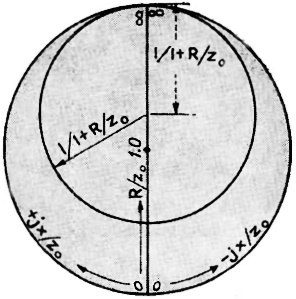
Construction Data
The data for construction of the main impedance coordinates of the calculator
is shown in the figure. It will be seen that all of the circles of constant resistance
are centered on the resistance (R/Z0) axis between the limits where R/Z0
= 1.0 and ∞ and that these circles are all tangent to the edge of the coordinate
system at the point when R/Z0 = ∞.
The circles of constant reactance are all centered along a straight line perpendicular
to the R/Z0 axis at the point where R/Z0 = ∞.
The scales along the radial arm of the calculator are conveniently plotted as
a function of the magnitude of the voltage reflection coefficient k (a linear scale
running between 0 at the center and 1.0 at the rim). The formulas utilized are:
Minimum Voltage or Current (N):
k = 1 - 2/(1 + (1/N2) )
(13)
Maximum Voltage or Current (X):
k = 1 - 2/(1 + X2)
(14)
Standing Wave Ratio (db):
k = 1 - 2/(1 + log-1 db/20)
(15)
Standing Wave Ratio, greater than unity (SWR):
k = 1 - 2/(1+SWR)
(16)
Attenuation (db):
k = 1 - (2 tanh (0.11512 db) / tanh (0.11512 db) + 1)
(17)
Standing Wave Loss Coefficient (C):
k = 1 - 2/(1 + C + √(C2 - 1)
(18)
Reflection Loss in db:
 (19)
(19)
Arrangements have been made with the Emeloid Co. of Arlington, N. J. for manufacturing
and marketing the radio transmission line calculator in durable plastic.
* Smith, Phillip H. Transmission Line Calculator, ELECTRONICS, January 1939.
** Morrison. J. F., Transmission Lines, Pickups (Western Electric Co., New York,
December 1939. See also "Radio Engineers Handbook," Terman, p. 174.
Posted July 10, 2023
|
")


