|
December 1964 Radio-Electronics
 [Table of Contents] [Table of Contents]
Wax nostalgic about and learn from the history of early electronics.
See articles from Radio-Electronics,
published 1930-1988. All copyrights hereby acknowledged.
|
Phase, feedback, and instability,
which happens to be the title of this 1964 Radio-Electronics magazine article,
has never been my forte. The controls course I had in college was one of the most
challenging of all, along with semiconductor physics. For some reason, I had trouble
figuring out how to construct the formulas properly in the more complex systems.
It was an intensive exercise in applying
LaPlace transforms. Controls
class was one of the very few courses in which I did not receive at least an A-.
Anyway, the math presented in this article is very basic and will not be a stumbling
block to understating the basic principle of feedback. You cannot study feedback
and instability without being comfortable with a little geometry and trigonometry,
so be prepared. Author Crowhurst does not get into poles and zeroes in the right-half
and left-half regions of the complex plane, so that will prevent a few anxiety attacks
from his readers ;-)
Phase, Feedback and Instability - It's how you measure it
that counts
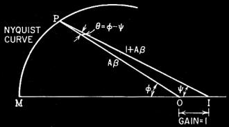
Fig. 2 - Basic construction of polar diagram for one frequency
that leads to the Nyquist curve.
By Norman Crowhurst
An amplifier design engineer phoned me, "I've made checks on the phase response
of our model XY-00 amplifier, and it shows less than 300 phase shift at either low
or high frequencies; but I receive complaints that under certain conditions the
amplifier is unstable. Is that possible?" Well, if he gets complaints, it must be
possible. Investigation showed he was laboring under one of the common misunderstandings
about the significance of phase measurements. Incidentally he had also square-wave-tested
the same amplifier, with excellent results, but got complaints about the way it
handled transients.
The well known stability criteria for an amplifier with negative feedback (are
there any others, these days?) states that the gain of the amplifier must fall below
1 before the phase shift gets round to 180° at either low- or high-frequency
limits. It is based on the original work of Nyquist and Bode, but an essential feature
of this information often gets lost somewhere along the way. What usually is left
out is just how gain and phase shift are measured.
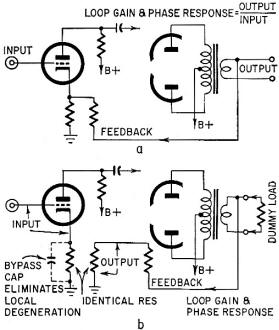
Fig. 1 - Difference between (a) normal method of measuring response,
gain and phase, of an amplifier, and (b) its loop gain and phase characteristic.
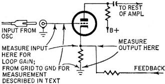
Fig. 3 - Measuring an amplifier's loop-gain response with feedback
loop closed.
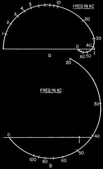
Fig. 4 - Nyquist curves with frequency marked: a-stable; b-unstable.
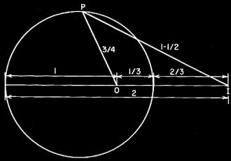
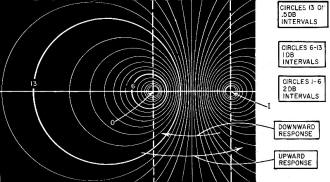
Fig. 5 (top) - Construction for one circle representing constant
input-to-output gain Aβ(1 + Aβ) = 1/2. (bottom) - A whole family of such curves
that can be used for determining overall frequency response from Nyquist curves.
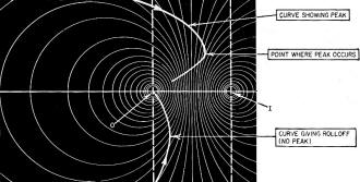
Fig. 6 - How direction in which Nyquist curve crosses pattern
of circles indicates nature of response curve and condition at peak, where one occurs.
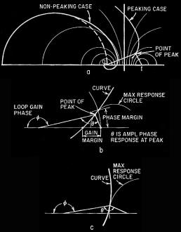
Fig. 7 - Criteria involving phase, relating to an amplifier that
peaks: a - a good shaping that avoids stability troubles: b - same part magnified
to show difference between peaking point found in phase analysis and the usual criteria
of gain and phase margins: c - a curve that represents an amplifier more likely
to give marginal trouble.
Our engineer friend was measuring it from input to output of the amplifier, complete
with its feedback loop closed (as you would buy it, in fact) (Fig. 1-a) . Unfortunately,
the important criteria concern the response from the input of the amplifier without
feedback, through to the output and back through the feedback loops ready for connecting
to the input again (Fig. 1-b). This is a very different thing.
Before we dive in to make measurements, let's take a closer look at the circuit
to see what we should expect. It can be made simpler to understand by using the
kind of vector diagram that builds into the curve first introduced by Nyquist (Fig.
2). Basically the Nyquist curve is plotted by using points (such as P) that represent
the amplifier's loop gain, measured as just described. This is represented by the
product A(3, or the length OP, in which quantity A is the amplifier's forward gain
(from input to output), and (3 is a fraction corresponding to the amount fed back.
I or OI is the input signal.
This can be measured, even with the feedback closed (provided the amplifier is
stable that way and does not oscillate) by measuring the input between grid and
cathode (not ground) and the output between cathode and ground (Fig 3). If the feedback
is through a simple resistor (without any fancy "phase-compensating" capacitors),
the cathode-to-ground voltage will be a scaled-down version of the output, but the
input is still different from the normal amplifier input.
This loop gain can be plotted either as two separate responses, one for magnitude
and one for phase, or the information can be combined in a single Nyquist diagram,
if desired, noting the frequencies along the curve (Fig. 4-a). In the Nyquist presentation,
the magnitude and phase of the loop gain are given by OP and Φ, respectively
(Fig. 2). For any particular frequency, the Nyquist diagram, with a little construction,
will tell us about other phase and magnitude relationships.
The important thing about the diagram (known as the Nyquist criterion) is whether
the curve stays "inside" point I, as at Fig. 4-a. Here, although the feedback gets
to be positive instead of negative just above 40 kc, it is not enough to equal the
input (OI), and hence the amplifier is stable. If the curve goes around point I,
as in Fig. 4-b, the positive feedback at just over 40 kc is more than the original
input and the amplifier will oscillate. But let's see what else we can learn from
this diagram.
The original input (between grid and cathode) is represented by the unit length
OI (Fig 2). The fed-back signal is out of phase, ideally, with OI, and starts at
OM. But amplifier phase shift, Φ, brings it to the value represented by OP.
So the actual input needed for the amplifier with its feedback loop closed will
be the remaining side of the triangle, IP. Thus the difference between the amplifier
input as seen from the outside and as the amplifier sees it, because of its feedback,
is represented by IP and ψ in magnitude and phase. Using I as the center or
reference point instead of O, the same Nyquist curve can be used to show the actual
input needed to get an effective input OI.
Now, if we connect our gain and magnitude measuring equipment so the input is
measured in the usual way, grid to ground, while the output is measured from cathode
to ground (also shown in Fig. 3), the input quantity is represented by vector IP,
while the output quantity is represented by OP. The magnitude of this "gain" will
be the ratio between IP and OP, while the phase angle measured will be the difference
between Φ and ψ, or θ.
If the feedback is just a resistance, then the amplifier output will be a "scaled-up"
version of OP, before it is cut down by fraction β, and the angle θ will
be the phase between input and output of the whole amplifier, complete with feedback.
Notice that, while the angles Φ and ψ get relatively large, the angle θ
remains quite small. This is the angle our engineer friend assured us stayed within
30°.
Gain is a little difficult to visualize as the ratio between the lengths of two
lines, but there is a fairly simple way to make it easier. If we find all the points
for P, such that IP is twice OP, which would mean the loop gain with feedback included
is -6 db, they will lie on a circle (Fig. 5). Similarly, all the possible points
for any other specific ratio of IP to OP will make another circle.
It is relatively easy to draw a whole family of circles, each representing a
specific value of possible overall gain (as measured on the complete amplifier rather
than loop gain). In this way, the same Nyquist curve can now be used to read off
overall gain, with feedback closed, except that the output used is after it is fed
back to the input, while the actual output is obtained before the feedback cuts
it down by (3. But if this is a simple resistance, the relative gain is accurately
given in this way.
Now we can visualize, with this diagram, how feedback works to produce peaking
in the loop-gain response (with the loop closed) as well as merely to find out whether
the amplifier is stable or not, by whether the curve goes outside or inside the
point 1. Fig. 6 represents a magnified section of a Nyquist curve plotted against
the circle background in the region that determines the rolloff characteristic.
If the curve pushes outward over the pattern of circles, this represents a rising
response, toward a peak, while if the curve goes inward through the circle pattern,
toward its ultimate destination at O, there is no peak, just a smooth rolloff.
With this method as an aid, we can further investigate what to expect from a
practical amplifier. If the amplifier has been well designed, so one internal rolloff
acts well before all the others, the Nyquist curve will start out as a slight departure
from a semicircle, finishing up with a tiny spiral (Fig. 7-a).
Each stage, or coupling, in an amplifier causes at least a high-frequency rolloff,
or turnover, due to circuit self-capacitance beginning to bypass the circuit's basic
impedance. Stages where a coupling capacitor is used will also cause a low-frequency
rolloff or turn-over, which occurs where the reactance of the coupling capacitor
becomes equal to its associated circuit impedance. The performance of the amplifier,
as shown in its Nyquist curve, is determined by how these turnovers combine, as
fixed by choice of circuit values.
For example, one low-frequency rolloff may be at 20 cycles while the remainder
are all below 2 cycles. Similarly, one high-frequency rolloff may be at 20,000 cycles
while the others are above 200,000 cycles. If this arrangement uses enough feedback
to produce a peak, the point where it reaches the peak, represented by the farthest
"out" in the pattern of circles, will be where the angle θ between OP and
IP is in the region of 90°, while the angle Φ will be between 135° and
180°. This is the point where the amplifier comes nearest to being unstable
and where transients may cause ringing.
Notice that it is different from either the gain margin or the phase margin (Fig.
7-b), as normally defined. It falls at a frequency between them. Gain margin is
the amount ("spare") between the point where the curve becomes purely positive feedback,
represented by crossing OI, and point I, where it would just oscillate. Phase margin
is the angle short of the 180° needed to make the feedback pure positive, when
the gain around the loop is just 1, shown by the radius from O being equal to OI.
Gain and phase margins are idealized quantities difficult to identify in practical
measurements, but this peaking point is easy to locate. It is where amplifier gain
is highest.
Sometimes amplifiers are designed, either deliberately or unintentionally, so
several rolloff's act more or less together at the same turnover frequency (say,
all of them start at 20 and 20,000 cycles). In this case the Nyquist curve will
deviate much more from the original semicircle, so as to swing inside point I at
quite a different angle (Fig. 7-c). This kind of design usually means the gain margin
is rather small, and likely to take trips into oscillation under certain circumstances.
Also the phase angle θ where peak occurs will be much bigger than 90°
and getting nearer to 180°, more like the angle Φ in this case.
Now we have some information we can use in taking amplifier response characteristics.
Instead of looking for the 180° point we need to pursue the response out to
a peak, if there is one. If the phase angle at this peak is in the region of 90°,
the amplifier is inherently stable, but it has a peak that may spoil its transient
performance. But if the peak occurs nearer to 180°, even though the peak is
not a very high one, the amplifier could be unstable in places.
So far we have assumed that the feedback does not use any "phase-compensating"
capacitors - at least not in the feedback circuit. If it does, then we cannot use
the output voltage compared directly with the input voltage. What we need to compare
is the fed-back voltage with the input voltage (Fig. 3). This is what we shall do
in the next article of this series.
Posted February 28, 2024
(updated from original
post on 2/28/2024)
|