Imaginary Numbers Are a Cinch
|
|
Mathophobes beware; I cannot be held accountable for instances of hyperventilation, fainting, intense sweating or nervousness, post traumatic stress, etc. When in high school and junior high, I suffered from the common malady. However, after setting my sights on earning an electrical engineering degree, I embraced mathematics as a necessary skill to be successful. In fact, I did very well in all my math classes even up through calculus, differential equations, and even higher levels. It soon became evident that my fellow students who struggled the most - even failed - at engineering courses were those who never had a handle on math. Since becoming comfortable with higher mathematics, my appreciation for its abilities to describe the physical world has constantly grown. It is also nice when reading technical articles to at least somewhat understand the math behind the concepts. Author Norman Crowhurst attempts in this 1960 Radio−Electronics magazine article to sooth the pain of complex numbers a bit. Imaginary Numbers Are a Cinch
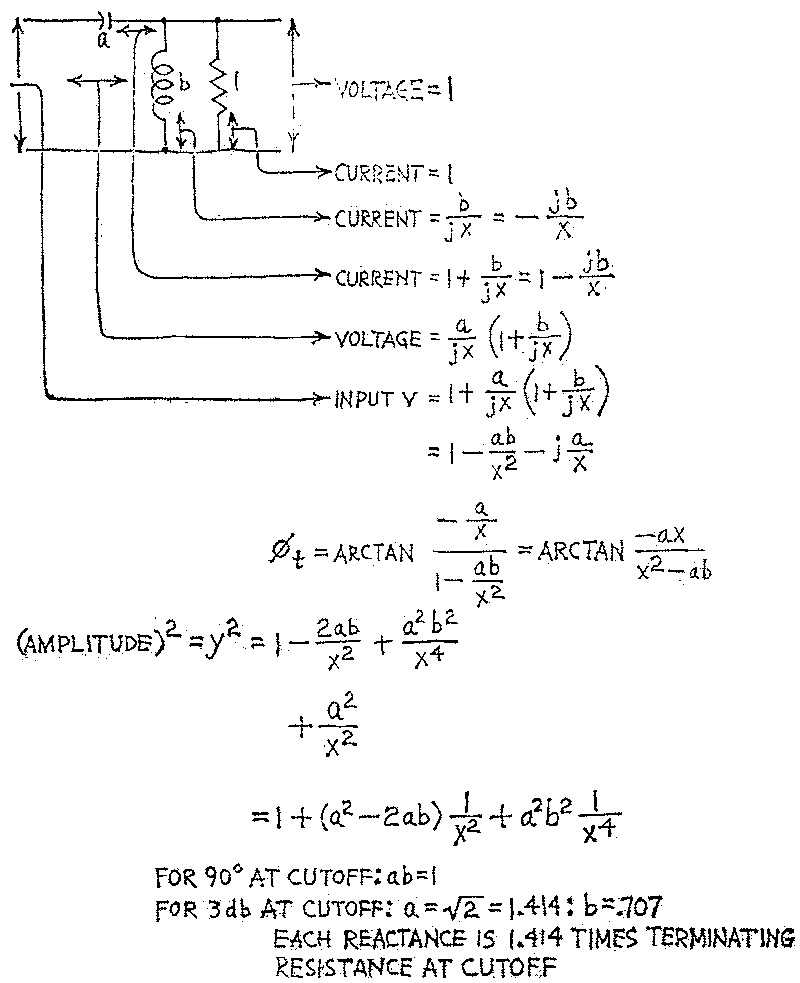
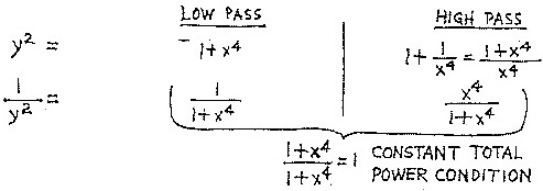
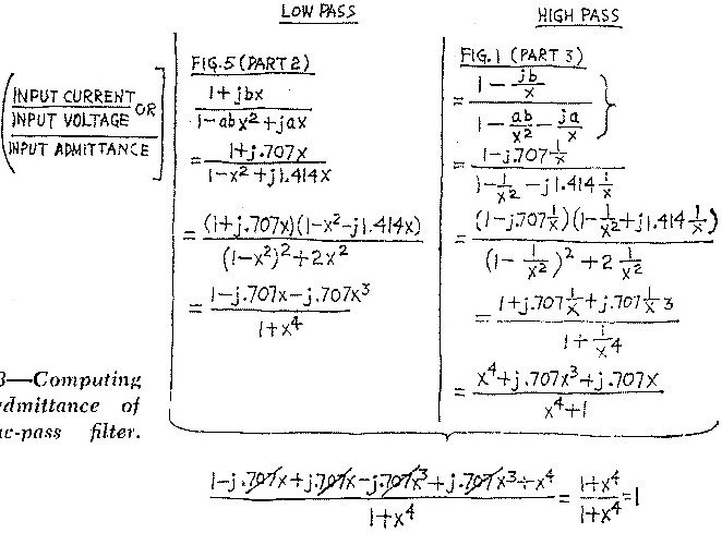
Fig. 1 - Diagram of high pass filter, and what it does in simple math terms. Want a low- or high-pass filter? Find out how to design your own By Norman H. Crowhurst When I next dropped by George's lab, he'd been doing his homework on imaginary numbers. He'd made a neat tabulation of all the results he could find about the simple two-element low-pass filter we had been working with and started extending it to a three-element type. Now he wanted to know more. "I think I could go ahead with more complicated low-pass filters, with a little trial and error," he said. "I suppose you can apply the same method to high-pass filters, but I couldn't see it." "Let's just reason it out as we did for the low-pass." I sketched a high-pass circuit and started translating its performance into an equation (Fig. 1). "The output is an inductor in shunt with the terminating resistor, and its normalized value is unity. Ee let the inductive reactance be represented as b units at cutoff frequency, as we did with the shunt capacitor of the low-pass filter. Should these units represent reactance or susceptance really, at cutoff frequency?" "That's what had me stymied," admitted George. "You can use either, with the proper care," I went on. "I find it simpler to use susceptance for all shunt elements and reactance for all series elements. Then we show its variation with frequency and phase of the elements by where we write x and j." "So the susceptance of the inductor will be jb/x?" queried George, who had obviously been thinking about this. "Last week we set a standard about phase for this kind of calculation," I reminded him. "It was that a + j means the quantity leads the reference quantity. Here, reference quantity is voltage across both the output resistance and the shunt inductor, so the j applies to the inductor current." "And current lags voltage in an inductance," went on George, "so it should be -j, right?" "Right. But an easier way is to just remember that the j and x always go together; this automatically takes care of the sign." I showed him that b/jx is the same as -j(b/x). He was already figuring out the expression for this high-pass filter. George was taking to the use of j like a duck takes to water. In short order, he had the phase and amplitude expressions figured out, as well as values for a and b for the constant-resistance type. He set these down alongside those he had tabulated for the low-pass unit. "Hey," he said, "the values and, when you make ab = 1, the phase angles are the same for both, except for the sign. What does that mean?" "Simply that the transfer phase of these two filters is 180° apart at all frequencies, when they use the same cutoff frequency as in a crossover." "Can you also show from this that a crossover like these makes constant resistance and delivers constant total power?" "For power, take the reciprocals of the amplitude-squared expressions, and add them," I suggested, which he did (Fig. 2) almost as quickly as I said it, and found the answer reduced to 1/1. "Does that prove the constant-resistance property as well?" "Not directly, you need to figure out the input admittance of each filter and then ado the two together." I showed him step by step how to do this for the low-pass (Fig. 3). He did the same for the high-pass, converted to x instead of 1/x as the variable in this case, added them, and found the sum was again equivalent to 1/1. "Show me a three-element low-pass design," George asked. I drew the design (Fig. 4-a). I put in a, b, and c to represent the normalized reactance and susceptance of the elements at cutoff, and we started figuring. "The voltage across the output inductor is jcx," said George, "so the total voltage at the mid-point capacitor is (1 + jcx) , isn't it?" I nodded, so he went on, "Then the current through the capacitor is ..." and he wrote it out: jbx (1 + jcx). "Now what?" "What's the current through the input inductor?" I suggested.
Fig. 2 - Power condition of the network.
Fig. 3 - Computing Input admittance of the low-pass filter.
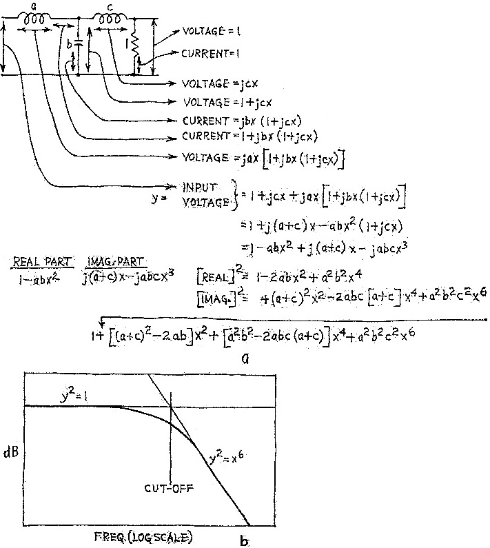
Fig. 4 - Design (a) of low-pass filter and the graph (b) of its performance.
Fig. 5 - How to make X2 and X4 disappear.
Fig. 6 - Changing slope curve by calculus.
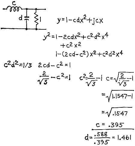
Fig. 7 - Transform math into a filter.
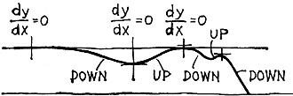
Fig. 8 - Movement of point on a curve.
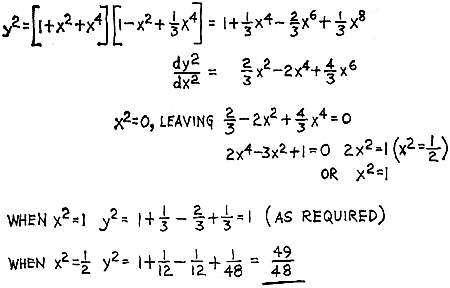
Fig. 9 - 0verall amplitude-squared math expression. "It's the current through the capacitor, plus that going to the output - is output current 1?" he asked. I nodded, so he wrote, for current in the input inductor: 1 + jbx(1 + jcx). "Then the voltage across the input inductor is ... and he wrote out: jax {1 + jbx (1 + jcx) }. "Now you just add the voltages together to get the input voltage," I suggested, sketching in the voltages on the schematic. By this time George was working it, to come up with the answer: 1 + jcx + jax {1 + jbx (1 + jcx) }. "Yuk," he commented, so I took over and removed the parentheses, till we had: 1 - abx2 + j(a + c)x - jabcx3 "Now what?" asked George. "Just solve for a, b, and c, I suppose you'll say." "That isn't as difficult as you might think, for the constant-resistance or maximal-flatness case. First, let's figure out the amplitude-squared expression." George squared the real and imaginary parts and added the terms in x2 and x4 to come up with 1 + [ (a + c)2 - 2ab ] x2 + [ a2b2 - 2abc(a + c) ] x4 + a2b2c2x which evoked another "Yuk !" when he'd finished. "Well, we can simplify that somewhat," I said. "First we want the rolloff asymptotic to cutoff, so the coefficient of x6 must be one." "Come again," said George, confused by the abstract math terms. So I sketched out the response on log/linear paper (Fig. 4-b). I explained that the 1 of the amplitude-squared expression represents the horizontal part of the response in the passband, while the x6 of the last term represents an 18-dB-per-octave slope, crossing the zero line at cutoff frequency. "So that means abc must equal 1." George promptly made that substitution by crossing out abc and a2b2c2. "Next, for maximal flatness, the terms in x2 and x4 have to disappear," I told him. "So the whole thing boils down to just (1 + x6)?" asked George, and added, "Oh, I see now what you meant by its being asymptotic." I nodded. "'The curve approaches a straight line, but never quite gets there." "That's negotiable," he said, writing out (a + c)2 - 2ab = 0 for x2 and a2b2 - 2(a + c) = 0 for x4 (Fig. 5). Then he looked stumped. "Because abc = 1, how about writing 1/c for ab?" I suggested, which he immediately did. "From the x4 equation, 2(a + c) = 1/c2, so (a + c) = 1/2c2, right?" he asked. I nodded. "So I can substitute this in the x2 equation to find c?" He was doing it and came up with the conclusion c = 1/2, followed by ab = 2, then a = 1.5, and finally b = 4/3. "Now we know the coefficients, let's look at phase," I suggested. George had the expressions for y, y2 and Φt with values of a, b and c substituted to give a simple numerical result (Fig. 5). "One element shifts 45° at cutoff, two elements make it 90°, does the third element shift it to 135°?" He crossed out the x's in the arctan expression and found it simplified down to -1, which is the tangent of 135°. Then he spotted that 90° would be where the denominator is zero, or x2 = 1/2 and x = 0.707, while 180° would be where the numerator is zero, or x2 = 2 and x = 1.414. "The whole thing looks easier by the minute," he commented. "Don't bother with the high-pass section, I'll work that some other time, for my own amusement. What I want to get to is that filter you designed that started us off on all this. Can you show me that?" "Well, that's a little different," I admitted. "In the first place, all the filters we've discussed so far are 'ideal' designs: they are exactly what we want them to be - constant resistance, uniform total power. But there is no such thing as a perfect linear-phase filter, so we have to find what is the best we can do with a given number of components. Sometimes calculus will help, sometimes it's a matter for trial and error, with diminishing deviations. So I think we should look at that kind of problem first." "Oh yes, you were going to show me how calculus helps," George commented. "Can you give me a quick example?" "Calculus deals with slopes," I explained. "It's not too easy to work out for phase response, but it's easy with amplitude response and we use the same principles for phase. Suppose you have a response with rolloff something like this," and I sketched it out (Fig. 6). "Detailed analysis shows its amplitude expression is of the form (1 + x2 + x4) which yields a 4.77-dB loss at the 90° point, where x = 1. Suppose we want to add a circuit that will reduce the loss to zero at this frequency, with minimum deviation up to this frequency." "Sounds difficult. How do you go about it?" "First step is to cook up the required overall amplitude-squared response, for which two requirements will set maximum flatness: boost equaling attenuation at x = 1 (4.77 dB for both); and, slope at the same point equal and opposite to that of the existing circuit, both measured on a dB/log frequency scale." I sketched in how this worked. "As we're interested in frequencies up to the normalizing point of x = 1," I went on, "it's easy and useful to work in that reference, and find out how good the result is when we get through. The attenuation of 4.77 dB (log 3 = 0.477) merely means that 1 + x2 + x4 is 3 when x = 1 (which is fairly obvious). We use a two-reactance filter that provides a peak before rolloff, which means its amplitude response will be of the form y2 = 1 - ax2 + bx4. We must solve for the two conditions: boost equal to attenuation, and equal, but opposite slopes; both at x = 1, to find a and b. Then we can convert this information into a designable filter circuit, by use of the j operator." "I get the idea," said George, "but it's not all clear yet. For boost to equal attenuation, the amplitude-squared expression should be the reciprocal at x = 1, shouldn't it?" I nodded. "So (1 - a + b) must have a value of) 1/3," he went on. "But how do you figure out the equal-slope part?" "That's where calculus comes in," I replied. "The slope we are interested in is plotted on log frequency and log amplitude (dB) scales, so the slopes we want are expressed by (d log y)/(d log x), writing y for the amplitude. Because we use expressions for amplitude squared, it's easier to work in y2 and x2 as variables, so we'll use that form." Showing him the standard differentials in a handbook he had, I wrote the conversion
For the first expression, y2 = 1 + x2 + x4. I figured this out to
Making x = 1 reduces this to a simple 3/3 = + 1. For the expression y = 1 + ax2' + bx4, the slope figures out to Making x = 1 in this expression reduces it to (-a + 2b)/(1-a + b), which needs to be -1. So the equation for equal slopes may be written: a - 2b = 1 - a + b, which rearranges to 2a - 3b = 1. And the amplitude requirement equation reduces to a - b = 2/3. George soon had these solved, to a = 1, b = 1/3. "But how do you make that into a filter?" he wanted to know. "Assume it's of this configuration," and I drew it out (Fig. 7), using c and d as constants for the inductor and capacitor. "Then you solve for values of c and d that make the amplitude-squared equation come out to y2 = 1 - x2 + 1/3x4." George was glad of the exercise in using j and in short order had equations in c and d that made a = 1 and b = 1/3. Together we solved them, using a slide-rule to get approximate values of c = 0.395 and d = 1.462. Using the reciprocal of d, which is 0.685, we could use a reactance chart to design such a filter for any terminating resistance and cutoff frequency. "How good is the correction this filter makes?" George wanted to know next. "We can use calculus for that too. The maximum error will be a stationary point on the graph of the amplitude-squared equation, which means the slope of the graph is zero." I sketched this. "Just a minute there," interjected George, "you've lost me, momentarily." I showed him (Fig. 8) that a point moving along a curve can go up or down; or it can momentarily do neither, in which case it is stationary at the top of a peak or at the bottom of a dip. I pointed out that an amplitude-squared response with terms in x2 and x4 can have one stationary point (a peak) if the coefficient of x2 is negative. Thus, the combined response after "correction" can have three stationary points, one at zero frequency, followed by a dip and a peak before final roll off. "To find these points, we differentiate the amplitude-squared expression, for convenience using x2 as the variable rather than x, and equate to zero (for zero slope). "The overall amplitude-squared equation is ... " George began, when he'd grasped this, and he wrote it out to y2 = 1 + 1/3x4 - 2/3x6 + 13xs. I differentiated it (not bothering with log terms, because a stationary point has zero slope no matter which scale is used) and got (see Fig. 9) Equating this to zero, x2 must be zero, or 1/2, or 1. The point at which x2 = 1 is the point for which we designed, s the point where x2 = 1/2, at 0.707 below cutoff, represents a dip. Substituting x2 = 1/2 into the amplitude-squared expression gives the fraction 49/48. Taking 10 times the logarithm of 49/48 gives the deviation in dB as 0.089. George was impressed with how small a deviation this correction could achieve - less than 0.1 dB. Before I left, he wanted to know what else operator j could be used for. I suggested it could be used to analyze anything that uses vectors. We had discussed vector analysis before. George was convinced his new knowledge of how to use operator j was going to prove a very useful tool. R-E
Posted April 21, 2023 |
|