How to Use Radio Propagation Predictions
|
|
Short wave radio was a boon to both professional and amateur radio operators because of its ability to be received over longer distances using significantly lower transmitter power. In 1947 when this article appeared in Radio-Craft magazine, the problem was (and still is) that short wave bands typically suffer from atmospheric ionization effects that vary depending on time of day, local weather, solar activity, pollution, and other phenomena. Long wave's advantage was that although it required higher power and longer antennas, it was (and is) extremely reliable. For other than the most critical applications, idiosyncrasies of short wave communications were accepted as the price of more convenient and lower cost operation. Widespread adoption of short wave communications brought extensive studies and characterization of atmospheric influences in particular frequency bands. Discovery of distinct "F" layers (regions) in the ionosphere and their effects on radio transmission has allowed radio operations to predict and accommodate the affected propagation paths. What does the "F" in F-Layer mean? According to my sources the "F" refers not to frequency, but to "free" electrons in the ionosphere. Here are a few really nice propagation prediction website that give up-to-the-minute data: HamQSL.com, ARRL.org, DX.QSL.net, VOACAP.com, DXZone.com, SolarHam.org How to Use Radio Propagation Predictions
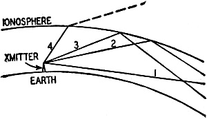
The various layers of the atmosphere. Though all affect radio transmission at certain frequencies, F-layer reflections are most important for long-distance communication. Scale at left in miles. By Fred Shunaman Old-timers remember when the best radio wave was the longest one. The long wave was reliable. It maintained the same strength day and night at all times of the year, and the strength dropped off steadily with increasing distance from the transmitter. Short waves - roughly those under 1000 meters - were "unreliable." They varied in strength with the time of day and the season and showed other "unpredictable" vagaries. The reliability of the long waves was obtained at the cost of high power. With the coming of broadcasting, it was found that a station of a few hundred watts could be heard (when conditions were good, such as on a cold winter night) farther than a long-wave station of many kilowatts. Then the amateurs started to work at even higher frequencies, first on 150 meters (2 mc), then 80 (3.5 mc), later 40 and 20 (7 and 14 mc). At each increase of frequency they were able to transmit farther with less power. But other and more disquieting discoveries were made. A station which pounded in with ear-splitting volume one night might simply not be there at all the next. Amateurs found they were not able to communicate with old friends in the next state, but were being received solid several thousand miles away. Thus was "skip distance" discovered. One point was clear: if some way could be found to figure out these high frequencies, a new era in low-power, long-distance communication would open up. Scientists amateurs, and communications companies set out to learn more about these mysterious waves. First, the scientists Kenelly and Heaviside suggested that the upper parts of the atmosphere were ionized - that the ultraviolet rays of the sun break up the atoms in these upper regions where the air is so thin as to resemble a poorly exhausted vacuum tube - into negative electrons and positive ions. These upper regions of the atmosphere, they said, were filled with a partly conductive material, something like the interior of a gas-filled vacuum tube. This ionized layer reflected radio waves of high frequencies back to earth, but lower-frequency waves were merely absorbed by it. The higher the frequency, the farther the waves penetrated the layer; thus the greater the distance at which the reflected wave reached the earth (Fig. 1). Above a certain critical frequency, the waves keep right on through the layer and are lost to earth entirely. In 1923 the English scientist Appleton proved the existence of the Kenelly-Heaviside layer by beaming radio waves straight up and measuring the time the reflected waves took to return. He found that the higher-frequency waves took longer to come back, proving that higher frequencies penetrate farther into the layer. Height of the layer as measured by this earliest radar was about 70 miles. But as frequencies were raised toward 3 mc, the echoes suddenly disappeared - to return from a distance of more than 150 miles. Obviously there were two reflecting layers. Above 8 mc a double echo was noted, as if the higher layer were split in two.
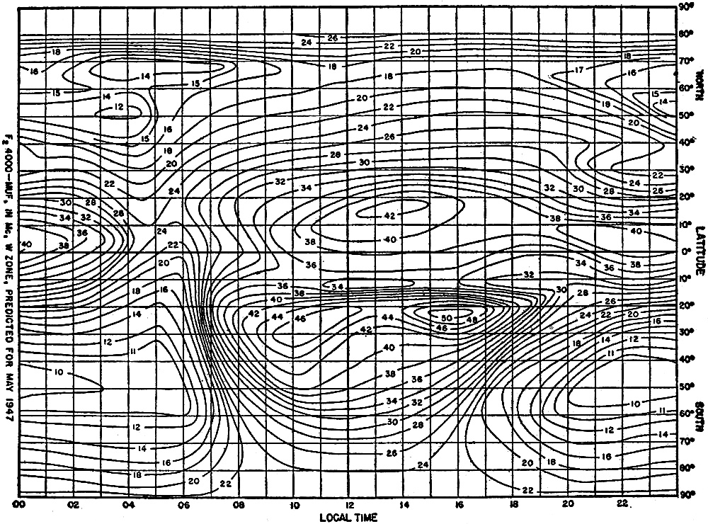
Fig. 1 - Long waves follow path 1, shorter ones, 2 or 3, and very short waves, path 4. The lower layer is now called the E-layer, and the higher one - or two - the F1- and F2-layers. The F2-layer is the most important one to long-distance, high-frequency communication. The E-layer is more important in daylight and at frequencies below 4 mc, though at times its effects may be felt up to 20 mc. Below these layers are the C- and D-layers, whose effects on radio waves have been little studied, but which are beginning to be considered important at certain frequencies. The Bureau of Standards at Washington has been one of the leading explorers of the ionosphere, and began in the late '30's to issue rough predictions of the probable ranges at various frequencies. The predictions were very approximate, and covered only four periods-summer and winter noon and midnight. The demand for reliable radio communication during World War II made much more detailed and accurate knowledge of ionosphere conditions necessary. Numerous stations were established at widely scattered points, and continuous records were made and transmitted to Washington for interpretation and correlation with those from other stations. These stations now number 58, and gather ionospheric data from all parts of the earth. The Central Radio Propagation Laboratory (CRPL) of the Bureau of Standards uses this information to issue monthly predictions of usable radio frequencies. These are put out in the form of monthly booklets, 3 months in advance. They contain maps and charts showing the maximum usable frequency for communication between any 2 points on the earth's surface at any time of day. The booklets are entitled Basic Radio Propagation Predictions and are used in connection with another publication, Instructions for the Use of Basic Radio Propagation Predictions (Bureau of Standards Circular 465), which contains further maps, charts, nomographs, and instructions for use with the Predictions. The Predictions consist of a series of charts of the ionosphere. Fig. 2 is one of them. The maps show the maximum usable frequencies (muf) for points at 4000 kilometers away from any point on the earth at any given time of day. Points on the same latitude do not have the same ionospheric conditions at the same time of day throughout the world. Therefore it is necessary to have 3 sets of charts. The western (W) chart includes South America, all the United States but the northwestern tip, most of Canada, the Atlantic Ocean and a bit of Africa. The eastern (E) chart is applicable to Asia and Australia, and the intermediate (I) to Europe, Africa, northwest Canada, Alaska, and a belt of the Pacific.
Fig. 2 - One of the ionosphere charts. There are six of these F2 and one E-layer chart.
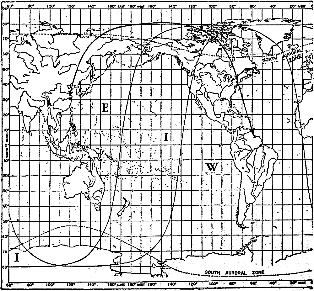
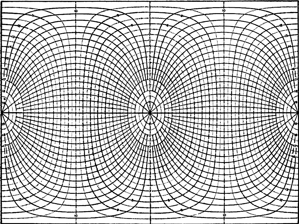
Fig. 3 - Part of the world map, showing the two great-circle paths mentioned in the text. Predictions Not Easy to Apply The Predictions are not particularly easy to use. It is often necessary to use 2 charts in conjunction, checking them against a third when the E-layer may affect results. A further difficulty is that radio waves follow great-circle paths, while the charts are square Mercator projections. This difficulty is solved with a great-circle chart in the Instructions. To use the Predictions, put a piece of tracing paper over the map of the world in the Instructions (Fig. 3). Mark the points between which communication is to be established. Also trace the equator line on the tracing paper. Then place the tracing paper on the great-circle chart (Fig. 4) with the equator lines coinciding, and slide it back and forth until one of the curved lines on this chart connects the 2 points. Draw the great-circle path between them along that line. Put the tracing paper on the correct ionosphere chart with the local station on the vertical line marking the local time of desired communication. Finding the correct frequency now depends on whether the distance is more or less than 4000 km (2500 miles). If the distance is exactly 4000 miles" the problem may be relatively simple. The mid-point of the great-circle path is located and the maximum usable frequency (muf) read direct from the F2 4000 chart for the given zone. For example, suppose contact is to be made between New York and Georgetown, British. Guiana, a distance of approximately 4000 km. The tracing paper is placed over the world map and the 2 points, as well as the equator, are marked on it. Then the paper is placed over the great-circle chart and moved back and forth till a great circle joins the 2 points. The path between the two is drawn, as well as the mid-point of that path. The tracing paper is then placed over the F2, 4000 W map with the equator lines again coinciding and the New York point on the hour meridian of the time desired. The muf of the mid-point is read. For example, in December 1947, the muf of the mid-point of the great-circle path between New York and Georgetown is 21 mc for 6 am, 34 mc for 12 noon, and 21 mc for 6 p.m. Since unpredictable conditions may cause the predictions to be in error, a frequency 15% lower than the. muf is taken as the optimum working frequency (owf). Thus all muf's are multiplied by 0.85 for actual working frequency. If the distance is greater than 400 km, 2 points 2000 km from each end of the path are taken instead of the mid point. The tracing paper is placed over the map as before and both points, as well as the equator, marked. The meridian of Greenwich may be drawn also, as a time reference. It is usually easier to use it for great distances than the local time of either of the 2 stations at the ends of the path. The great-circle chart is again used to find the actual radio path between the 2 points. Instead of marking the mid-point of the path control points 2000 km from the ends of the path are marked. (Experience has shown that muf's at great distances are little different than at 4000 km.) The maximum usable frequency for each of these points is found (on the appropriate chart) and the lower of the two taken as the muf for the entire path. For example, communication between New York and Shanghai is desired. Drawing the path and control point the muf's for the New York control point are found to be 28, 12, and 12 mc for 0600, 1200, and 1800 GMT, respectively. At the Shanghai end. using the F2 4000 E chart (not shown) all 3 muf's are found to be 12 mc. The muf for the whole distance is then 12 mc for the given times, and the owf 10.2 mc. For distances less than 4000 km a little more work must be done. The muf is first found exactly as for the 4000 km. Then the muf of the mid-point found on the F2 0 chart, which shows the critical frequencies for waves projected directly up from the sending station. Since the distance is between 0 and 4000 km, it might be expected that its muf would be between these two. And so it is, but in a way that does not vary directly with distance. A nomograph provided in the Instructions for distances less than 4000 km. A straight edge is placed between the muf at 0 and that at 4000 km, and the correct frequency is read where the straight edge intersects the line representing the distance of the station with which communication is to be established.
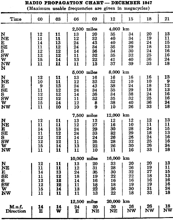
Fig. 4 - This great circle chart is used to find the radio transmission paths on Fig. 3. At lower frequencies the E-layer may enter into the picture. An E-layer chart in the Predictions helps the radioist to use reflections from that layer. After selecting the best frequency from the F charts, consult the E chart. If the E-layer muf is higher than that reflected by the F-layer, use the E-layer frequency. Adapting the Predictions All these methods are excellent for transmission between 2 fixed points, such as 2 commercial or government stations. They are not so good for the amateur or short-wave listener. The amateur wants to know what frequencies to use to cover a large area - possibly a continent - or in what direction to send a CQ to get results and dx on his transmitter's frequency. The short-wave listener would like to find out when to listen for elusive short-wave broadcasters. Both are on the alert for times when higher frequencies than those predicted are useful, for these are the periods of dx. A few attempts have been made to broaden the scope of the Predictions to cover amateur and general requirements. The most successful of these is based on the observation that a given muf "cloud" drifts along the earth from east to west, maintaining a constant angle with the sun. The amateur who works on 10 meters, for example, can note the area over which 30 mc or higher is the muf. If this area. covers the control points between him and any desired station, he can work that station on 10 meters. Another system calculates owf's for narrow strips along the American coast and that of other countries. The table presented here represents a new approach to the problem. Based on latitude 40 N in the western zone, a large number of calculations have been made, giving the optimum frequency for any part of the day for any distance and any direction. As conditions drift west with the sun, this chart will be correct for any part of the United States on the 40th parallel, and approximately correct for considerable distances north and south of that line.
Radio Propagation Chart - December 1947 (Maximum usable frequencies are given in megacycles) The table shows conditions at intervals of 3 hours and at ranges from 2500 miles (4000 km) to 12,500 miles (20,000 km) at intervals of 2500 miles. These intervals are close enough to permit interpolation for times and distances between those given. The same is true of directions. Use of the table is simple. The user merely consults it for the current hour and notes the optimum working frequencies in each direction for the various ranges. A combination of high working frequencies and great distance spells dx. Low frequencies in a given direction indicate the limits within which a receiver or transmitter should be held to work or hear from stations in those great-circle directions. A great-circle chart based on a point near the user's location is exceedingly useful for ascertaining the bearing of distant points. Less convenient is the chart published in the Instructions, but distances as well as directions can be obtained from it. A globe and piece of string is possibly the simplest means of finding direction and distance. For example, to find the muf for working between New York and San Francisco at 9 p.m. Eastern Standard Time during December, 1947, first find the bearing and distance by any of the means above. The distance is between 2500 and 3000 miles, and thus fits most closely the 2500-mile table. Bearing is a little north of west (in spite of the fact that San Francisco is south of New York). At 21 hours the maximum usable frequency west is 24 mc. For reliable work this should be converted to the optimum working frequency (owf) by multiplying by 85%. The owf is then about 20.5 mc. The nearest amateur band is 14 mc, though short-wave listeners may look for Treasure Island right up to its 21-mc frequency. Again, suppose a short-wave listener is interested in getting Shanghai or Nanking. Distance is ascertained to be approximately 12,000 km and the bearing slightly west of north. Looking at the chart, it appears that 13 mc at 9 p.m. offers the best opportunity, as read from the 7500-mile chart in the direction N. Checking with NW, the best times appear to be between 3 and 9 p.m., with a frequency as high as 33 mc at 6 p.m. However, the bearing is much more nearly north than northwest, leaving 9 p.m. the best hour. Only one direction is given for the 12,500-mile range, as it is the same distance in all directions. There is very little difference in muf over a wide angle from NE to NW. The operator with a rotatable antenna may find it worth his while to try various paths.
Posted April 11, 2024 |
|