Ground Resistance and Its Measurement |
|
An old electrician's saying goes "Ground is ground the world around*," implying that every point on Earth's surface is at the same potential - specifically 0 volts. We know, of course, that it is not so. Maybe on average such a claim could be made, but just as "sea level" is not the same at all points on the ocean's surface (hence we speak of "mean sea level"), neither is the voltage potential the same everywhere. Further, just as the salinity of all points on the ocean surface do not have the same salinity (and thereby conductivity), the conductivity of various places on dry land vary - often significantly. Electric power systems are very concerned with soil electrical conductivity in the vicinity of power generation (source), distribution stations (transmission lines) and end users (load). Soil conductivity measurements are made in critical installations and if necessary, multiple ground rods and/or even chemical enhancements to the soil are used to achieve the required values. Antennas likewise rely on a specific ground potential value to operate according to theoretical calculations (if a "perfect" ground is assumed). When a Yagi antenna is mounted on a mast at some physical distance above ground level, its feed point impedance and radiation pattern will come close to agreeing with its advertised performance specifications only if the ground underneath it sufficiently approximates a perfect ground. Achieving that type of ground often means running multiple copper conductors radially out from the support mast (usually buried, but not necessarily) and sinking ground rods. Modern electromagnetic field solvers easily and accurately predict antenna radiation patterns when the system model parameters are accurately determined and input. One of the most popular and affordable programs for amateur radio enthusiasts is called EZNEC (pronounced "easy neck"). EZNEC uses the NEC-2 (Numerical Electromagnetics Code ) calculating engine and allows the user to input antenna dimensions, soil conductivity, ground radials, antenna height, guy wires, nearby structures, and other relevant parameters. * A variation is "Green is ground the world around," referring to the nearly universal use of the color green for the insulation of a 'ground' wire. The National Electric Code (another, but different, NEC) does not specify a color for a grounding conductor; however, an equipment grounding conductor must be color coded green. Ground Resistance and Its Measurement
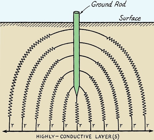
Fig. 1 - A ground rod has a large number of separate paths from it to one or more layers of the earth's crust. In this sketch each path is represented as having the same resistance, r, but this is not necessarily the case.
Table I By J. M. Bruning, K2BZ Proper operation and protection of electronic equipment usually requires that some part of the circuit be "grounded." Ground in this sense signifies an earth connection. The objective is to connect the apparatus through a low-resistance path to that portion of the surrounding earth - or water - which is highly conductive. A water-pipe ground is not always satisfactory, and a ground-rod system mayor may not operate properly. When trouble is experienced, the cause will usually be too high a resistance in the path between the pipe or rod and the surrounding earth. We must remember that the aim is to establish contact with that portion of the earth which is highly conductive. The better this objective is attained, the lower will be the ground resistance of the system. The conductivity of the earth depends upon the composition of the earth's crust, and is determined largely by the moisture content of the soil and by the nature and amount of raw or dissolved minerals in the soil. Considering these factors and the nonuniform distribution of rock, shale, sand, etc., it should be evident that the problem of establishing a low-resistance path to the earth is somewhat more complex than it ordinarily appears. Good practice decrees that the ground lead should consist of a fairly heavy copper wire securely fastened to the equipment and to the water pipe or ground rod. The inherent resistance of this part of the ground system is usually negligible, but there is no sure method for estimating the effectiveness of the over-all installation. While existing literature describes at length various ways to install a ground system, little information is available to explain how to compare the effectiveness of existing grounds or how one can quantitatively determine the amount by which a ground system is improved by soil treatment or by the installation of multiple rods. Ground Rods
Table I Each and every portion of the surface of a ground rod is connected through a separate path to one or more highly-conductive layers in the earth's crust, as shown in Fig. 1. Each path will have its own value of resistance, r. All of these paths are in parallel with each other, and the number of such paths is nearly infinite. Our problem consists of determining the joint resistance of a nearly infinite number of parallel resistors, each having an arbitrary and varying value of resistance. Skipping the mathematics, it can be shown that the summation for an infinite number of such parallel paths would be numerically equal to zero. This value of zero resistance is what we try to obtain in our ground system. While this figure cannot be reached, it can be approached. If the ground rod in Fig. 1 is increased in length, or in diameter, or if more rods are driven and connected in parallel, the number of parallel paths to the true earth will be increased and the resistance of the system will more closely approach zero.
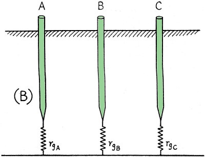
Fig. 2 - The resultant or effective resistance of the ground path can be lumped in a single value, rg in (A) Three separate ground rods might have different resistances to ground, as represented in (B).
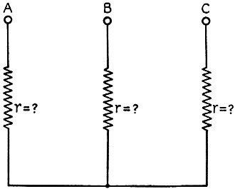
Fig. 3 - With three ground paths as in Fig. 2B, the calculation of anyone becomes a simple problem in algebra, since direct measurements can be made between A and B, B and C, and A and C.
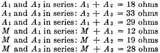
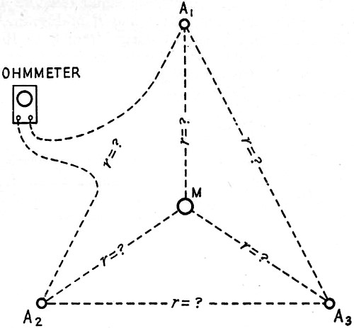
Fig. 4 - To measure the ground resistance at the rod M requires two or three auxiliary rods, A1 A2 and A3, and a series of ohmmeter readings of all possible combinations.
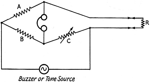
Fig. 5 - A simple Wheatstone bridge for measuring resistance in the presence of large earth currents. Resistors A and B should be equal and about 1000 ohms, and C should be a 100-ohm rheostat. R is the unknown resistance. Let us assume that the combined resistance of all the possible earth paths from a single ground rod can be represented by a single resistor, rg, connected from the bottom tip of the rod to a zero-resistance conductive layer in the earth, located some distance below the rod. The value in ohms of the resistor, rg, is the resistance to ground of the rod in question. This is represented in Fig. 2A. Any other ground rod may be similarly assumed to have its individual value of ground resistance, essentially unaffected by the presence of any additional rods, provided these other rods are placed a reasonable distance away. This is shown in Fig. 2B. For all practical purposes, the internal resistance of a rod having a diameter of one-half inch or more is negligible. Also, since one thousand feet of No. 10 copper wire has a resistance of about one ohm, it is apparent that a short and heavy ground lead between the equipment and the grounding system can have but negligible resistance. Thus our ground resistance is concentrated in the earth itself, and the additional circuit resistance of the rod and its connecting lead can be disregarded. We can now redraw Fig. 2B, leaving out unnecessary elements, as in Fig. 3. Solving for the Resistance Fig. 3 consists of three unknown resistors strapped together at one end. If these resistors were placed on a text bench and a technician were provided with an ohmmeter, he could determine the value of each resistance simply by connecting his meter to the terminals marked A, B and C. By reading the values for different combinations and doing a little arithmetic, he could easily determine the resistance of anyone unit. If, for example, a = resistance reading between A and B, b = reading between B and C, and c = reading between A and C, simple algebra proves that
In exactly the same manner it is possible to measure the ground resistance of any water-pipe or ground-rod system. Let us proceed to determine the ground resistance of a single rod. It will first be necessary to drive at least two and preferably three auxiliary test rods. These rods should be placed in a roughly symmetrical disposition around the master rod. Two test leads made of No. 14 insulated wire, terminated with heavy clips, will be needed to connect in sequence each two rods to an ohmmeter, as in Fig. 4. The series resistance of each pair of rods will be measured and recorded as in Table I. This table lists actual values measured on one ground system tested. The ground resistance of the master rod can now be found in the same manner used for solving the resistor network of Fig. 3. By using the readings for M, A1 and A2, one value for M can be determined. By similarly using M, A2 and A3 and M, A1 and A3, two other values of M can be found. Substituting the above figures, values for M will be found to be 6.5, 5.5 and 7 ohms. The average is 6.3 ohms. By similarly combining the indicated readings for rods A1, A2 and A3, we could determine their three values and their over-all average to be: Rod A1 = 7, 10.5, 6.5 = 8 ohms average Rod A2 = 11, 12.5, 12 = 11.8 ohms average Rod A3 = 22, 22.5, 21 = 21.8 ohms average The accuracy of the above readings can be estimated by noting how closely the three separate values agree. Any set of readings indicating a major discrepancy should be discarded and a new set of readings taken. Measurements should be made in opposite directions and the results averaged before tabulating. Rods should be driven a reasonable distance apart. Results have been found to be good if the separation is anywhere between ten and fifty feet. If the rods are too close, the accuracy of the readings may be affected. If too far apart, excessive ground potential may be encountered, causing the readings to fluctuate over a wide range. After rods have been driven there will usually be a gradual rise in resistance measurements taken over a period of a. few days as moisture and chemicals in the earth attack the surface of the rod. After several days this rise will taper off and subsequent measurements will remain relatively stable for fairly long periods of time. However, no ground system should be neglected for a period of greater than a year without rechecking the system's resistance. This should preferably be done in the spring of the year just before the lightning season, to insure adequate protection. Earth Currents In some locations the use of the d.c. ohmmeter becomes unsuitable because of large d.c. or a.c. components in the earth currents. For such cases the measurements can be readily made by using a Wheatstone bridge excited by a tone source of several hundred cycles or more and balancing the bridge for the lowest or null indication in a telephone headset indicator. This arrangement is shown in Fig. 5. If a Wheatstone bridge is not available, an acceptable substitute can be improvised by using two exactly equal resistors of about 1000 ohms for legs A and B in Fig. 5. A rheostat or pot having a range from 0 to 100 ohms can be substituted for bridge arm C, and the amount of resistance cut in by the rheostat at the point of balance determined by subsequent ohmmeter test. When the null indication is achieved, the bridge is balanced, and C is equal to the unknown resistance R. Variation of Ground-Rod Resistance with Depth Using the method described above, measurements were recently taken on a number of ground rods driven to a depth of twelve feet. These rods were used to form the grounding system for a steel tower erected in an exposed location. Due to the rocky and dry type of earth encountered, it was necessary to connect five rods in parallel to the central tower before the over-all ground system resistance was reduced to a reasonable figure.
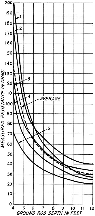
Fig. 6 - A graph showing the variation in resistance with rod length for five different cases. The variation decreases as the rods are made longer. Since the variation of ground resistance with rod depth is of interest, the actual values measured are plotted in Fig. 6. It will be noted from Fig. 6 that there was a wide range in the values measured for different rods at identical depths. This variation was most evident at shallow levels and decreased as the rods were driven deeper into the earth. At a six-foot depth the rate of decrease in resistance began to taper off. At ten feet all rods had a nearly uniform resistance. Readings at the twelve-foot level indicated that a practical limit had been reached. Driving the rods to greater depths would not decrease the obtainable resistances sufficiently to warrant the increased labor and expense. Summary The procedure given above enables a fairly accurate measurement to be made of the ground resistance of a rod, water-pipe or other grounding system. The measurement may be rapidly taken using conventional equipment in most cases. It would appear that in order to be effective and uniform from day to day, ground rods should be driven at least eight feet deep. However, the improvement achieved beyond the eight-foot level will taper off so rapidly that there is little point in sinking a rod below a twelve-foot depth. Still further improvement in reducing the ground resistance of a system can most simply be achieved by driving a number of rods to the desired depth and then connecting the rods in parallel, using heavy copper conductors. The grounding capability of any ground-rod system may be improved by conventional methods of treating the adjacent soil with dissolved rock salt or similar agent. However, the immediate improvement achieved may be at the expense of more rapid deterioration of the rod itself, necessitating frequent replacement. When available for use, brass pipe or copper-plated iron rod will give superior results from the viewpoints of initially low resistance and long trouble-free life. For really low-resistance ground systems totaling less than one ohm, an entirely different technique is called for. Cold water-pipe grounds should measure less than 20 ohms. Single ground rods may range from 20 to 500 ohms. When short rods are used or where dry soil is encountered, it may be necessary to parallel several rods. Of two grounds being compared, the one showing the lowest resistance usually will be superior in performance. Although satisfactory results may be expected if the measured ground resistance is below 10 ohms, every effort should be made to reduce this value as much as practicable. The reader is cautioned to note that this article has dealt exclusively with the "d.c." resistance aspect of a grounding system. The dissipation of r.f. energy in the ground is an entirely different matter. Where an effective r.f. ground plane is required at or near the earth's surface, the use of an elevated counterpoise or a buried radial system may be required. From the foregoing, it is evident that if a water-pipe or driven-rod system is to be used, the resistance of the system should be determined. The procedure described in this article will enable the required measurements to be accurately and quickly made.
Posted October 4, 2022 |
|