A.C. Calculations for Parallel and Series-Parallel Circuits
|
|
When you read a lot of tutorials about introductory electronics on the Internet, most are the same format where stoic, scholarly presentations of the facts are given. Those of you who don't have enough fingers and toes to count all of the college textbooks like that which you have read know of what I speak. When hobby articles are written in a similar fashion, it can quickly discourage the neophyte tinkerer or maybe even a future Bob Pease. The ARRL's QST magazine has printed a plethora of articles over the years that are more of a story than just a presentation of the facts. My guess is the reason is because often the authors are not university professors who have forgotten how to speak to beginners. This article on basic calculations for AC series and parallel circuits is a prime example. A.C. Calculations for Parallel and Series-Parallel Circuits Solving for Current at Voltage by Means of Admittance By S.E. Spittle, * W4HSG The problem of finding the resultant impedance of a group of impedances in parallel is not usually discussed in the more elementary texts on alternating currents, probably because the solution of such problems is rather lengthy and difficult without the use of complex algebra. The term "complex algebra" may have a mysterious and rather terrifying sound to those who have never heard of it, but actually the process is comparatively simple for anyone having a knowledge of the elements of plain algebra.
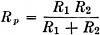
Fig. 1 - Parallel resistances. The recent QST article entitled "Meet Mr. j"1 provides a good explanation of the application of complex algebra to alternating-current circuits and should be read as an introduction to this discussion. In that article one method of computing the impedance of parallel circuits by means of their phase angles was described. An alternative method, described here, makes use of the resistive and reactive components without requiring a knowledge of the phase angles as such, and therefore can be applied without the use of trigonometric tables. Since the laws of alternating-current circuits are merely extensions of the laws governing direct-current circuits, taking into account the effects produced by the storage of energy in the electric and magnetic fields, it is logical to explain the solution of a.c. problems in terms of the familiar operations used with d.c. problems. For example, take a circuit consisting of two resistances, R1 and R2 in parallel, as shown in Fig. 1. I1 = EG1 I3 = EG3 I2 = EG2 Ip = EGp The usual formula for finding the parallel resistance of this combination is
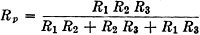
However, this formula is only a special case of the more general formula 1/Rp = 1/R1 + 1/R2 + 1/R3 ... etc., applied to the case of only two resistances. In the special case of two resistances, the second formula is converted into the first by means of a few simple transpositions; When there are more than two resistances, the general formula is more practical, as will readily be seen if we apply the same process to the case of three resistances. Thus 1/Rp = 1/R1 + 1/R2 + 1/R3 when transposed becomes
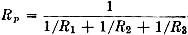
It may be interesting to note that the process of finding the resulting resistance is the same as finding the total current in the parallel circuit, using any assumed value of applied e.m.f. Thus Ip = E/Rp = E/R1 + E/R2 + E/R3. Changing the value of E will change Ip but not Rp. Therefore we can assume E to be one volt, giving the formula for the parallel resistance, which is usually expressed as
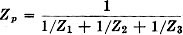
The same formula can be applied to a number of parallel impedances in an a.c. circuit, giving
The catch in this is that the currents in the various impedances are usually not in phase with each other, so that the phase difference must be taken into account in obtaining the correct value of parallel impedance. In the d.c. case the quantity 1/R is known as the conductance, represented by G whose unit of measurement is the mho. Thus, a resistance of 5 ohms corresponds to a conductance of 1/5 or 0.2 mho. The total conductance of a parallel circuit is the sum of the conductances of the individual branches. Thus, making 1/R1 = G1, etc., we have for three resistances in parallel Gp = G1 + G2 + G3, and the equivalent or parallel resistance, Rp, is equal to 1/Gp. The conductance, G, is numerically equal to the current which would flow with one volt applied to the circuit. Hence, in finding the total conductance of a parallel circuit by adding the individual conductances we are merely following the same process as in finding the total current by adding the individual currents. If this can be done for d.c. circuits we should likewise be able to do the same thing for a.c. circuits. In the latter case, 1/Z is called the admittance and is represented by Y. Also, the total admittance of a parallel circuit is Yp = Y1 + Y2 ... etc. The value of Y is also measured in mhos, just as resistance, reactance and impedance all are measured in ohms. Here we remember our forgotten friend, the phase-angle. We know that if we apply an alternating voltage to a circuit having several parallel branches, the absolute values of the branch currents will add up to more than the absolute value of total current unless all the currents happen to be in phase. Since the admittance is a measure of the value of current that would flow in an impedance when one volt is applied, it is necessary to add admittances in the same manner as we add currents in a parallel circuit. The only practical ways of adding a number of currents, voltages or impedances having various phase angles are by drawing scale diagrams or by splitting each one into two components at right angles to each other, adding the two sets of components separately and then combining the two sums by the familiar right-triangle rule, or Pythagorean theorem. One component represents the condition of current in phase with voltage, or 100 per cent energy consumption, and is often called the real component . The other component represents the condition of current and voltage 90 degrees out of phase, or 100 per cent energy storage, and is often called the imaginary component. This component is usually prefixed by the letter j to show that it has been rotated 90 degrees with respect to the real component. The letter j has been given the value of √(-1) and when it occurs in a computation it is treated as a multiplier having this value, as has already been explained in the article mentioned previously. Algebraic numbers having √(-1) as a factor are known as imaginary numbers, which explains the name given the components of voltage, etc., to which the letter j is applied. The method of adding the real and imaginary components of voltage or current also is covered very well by Mr. Noll and therefore only its application to parallel circuits will be discussed here. In many problems of parallel impedance the mathematical solutions can be simplified by the use of admittances. In this way frequent reference to trigonometric tables is unnecessary, since phase angles no longer are factors in the computations. Practical application of the method is discussed in this article and illustrated with typical examples. The preceding paragraph implies that we must split up each of our admittances into two components before we can add them. To obtain the components of the admittance we make use of the complex expression for impedance, which means the impedance when split into its components of resistance and reactance. Expressed thusly, Z = R + jX, the j means that, if a diagram of the components of impedance is drawn, the reactance, X, will be drawn at right angles to the resistance, R. Then, since Y = 1/Z, the corresponding admittance would be
In order to get the complex expression out of the denominator we multiply the fraction by
giving
since j2 = -1. Now we have
However, we know that R2 + X2 = Z2.
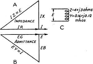
Fig. 2 - Impedance (A) and admittance (B) diagrams for the coil (C). In the impedance diagram, the current, I, is used as the reference, while the voltage, E, is used as reference in the diagram of (B).
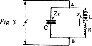
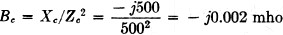
Fig. 3- RCL circuit. Therefore the two parts of the admittance, Y, are R/Z2 and - jX/Z2. If Z happened to be a pure resistance, X would equal zero, and R/Z2 would become equal to R/R2 or 1/R, which is called G, or conductance in d.c. circuits. The term R/Z2 is therefore called the a.c. conductance and is also represented by the letter G. The term X/Z2, which is the reactive or imaginary part of the admittance, is known as the susceptance and is represented by B. Thus, Y = G -jB, where G = R/Z2 and B = X/Z2. Note that the phase angle of the admittance is of sign opposite to that of the corresponding impedance. 2 Fig. 2 shows an impedance diagram at A and the corresponding admittance diagram at B for a coil having 4 ohms resistance and 3 ohms reactance (C). The diagrams are shown in terms of the components of voltage and current, and an applied e.m.f. of 25 volts is assumed, so that both diagrams will be to the same scale. To find the resultant impedance of a number of impedances in parallel, we add the admittances of the individual branches to obtain the total admittance. The impedance of the combination is then the reciprocal of the total admittance, or Z = 1/Yt. The application of this method will be shown by a couple of examples. For the first example we shall take the tuned circuit of Fig. 3, consisting of a condenser of 400-μμfd. capacity with negligible resistance, and a 100-microhenry inductance coil having a resistance of 20 ohms. A circuit with these values will be series resonant at 795.58 kilocycles, as can be verified by the formula for resonance,
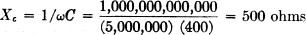
We shall now calculate the impedance of the circuit at this frequency, assuming a voltage to be applied between the points A and B, making it a parallel-resonant circuit. Since the factor ω = 2πf is used in calculating both inductive and capacitive reactances, we start by computing its value as follows: ω = (2) (3.1416) (795,580) = 5,000,000 (electrical radians). The impedance of the capacity branch is Rc - jXc Rc = 0 and
(There are 1,000,000,000,000 micromicrofarads in one farad). Therefore Z = 0 - j500 ohms. The admittance of this branch is Yc = Gc - jBc Gc = Rc/Zc2 = 0
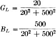
Therefore. Yc = 0 - (- j0.002) = 0 + j0.002 mhos. Since the impedance in this particular case is a pure reactance we could have found B directly, since 1/Xc = ωC. This short cut cannot be used, however, if the impedance also has a resistive component. The impedance of the inductive branch is ZL = RL +jXL RL = 20 ohms and XL = ωL = (5,000,000) (0.0001) henries = 500 ohms. so ZL = 20 + j500 ohms. The admittance YL = GL -jBL
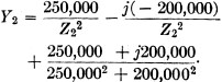
and
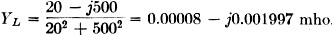
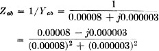
The admittance of the parallel circuit is Yab = Yc + YL = (0 + j0.002) + (0.00008 - j0.001997), which is added thusly, 0 + 0.00008 + j0.0002 - j0.001997 = 0.00008 + j0.000003 mho. The impedance then is
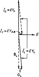
The result shows that the inductive and capaci-tive reactances in a parallel circuit do not cancel out in the same manner as they do in a series circuit. This results from the fact that the resistance in the inductive branch shifts the phase of the current slightly, so that it is not exactly 180 degrees out of phase with the current in the capacity branch. The current for a given applied voltage is equal to E/Z or EY, since Y = 1/Z. Therefore a diagram of the relative values and phases of currents in various parts of the circuit can be drawn by using the values of Y to represent the currents, since current is proportional to Y.
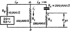
Fig. 4 - Vector diagram of the currents in the various branches of the circuit of Fig. 3. Fig. 4 is such a diagram, with the conductance and total current exaggerated to show the effect of resistance in the circuit. Actually the frequency at which the resultant reactance is zero is so close to the frequency at which XL = Xc that for all practical purposes they can be considered identical except in circuits having lower values of Q than are ordinarily used in radio work. Such low-Q circuits are, however, found in television amplifiers and are also likely to be found in audio-frequency work. A second example, illustrating a series-parallel circuit, is the resistance-coupled amplifier shown in Fig. 5. An exact calculation for such an amplifier, taking into account all possible current paths, is quite complicated, so that it is customary to reduce the amplifier to a simplified circuit which approximately represents the conditions existing for the frequency of interest. For low frequencies the circuit of Fig. 5 can be represented by Fig. 6, where the applied voltage is the a.c. voltage developed between plate and cathode by a signal, and is equal to μ times the a.c. voltage applied between grid and cathode. The voltage eg2 between grid and cathode of the following tube is practically equal to the voltage drop across the grid leak, since the voltage across the cathode bypass condenser is negligible if the bypass condenser has a fairly large capacity (considering the drop caused by the applied grid voltage only). This voltage will, therefore, be a portion of the voltage between A and B and will then depend upon the frequency as well as the constants of the circuit. Assuming the frequency of the applied signal to be 53 cycles per second, the reactance of the coupling condenser will be 200,000 ohms. With an applied signal of 1 volt and an amplification factor of 20 the amplified a.c. voltage applied to the network of Fig. 6 will be 20 volts. This voltage will be divided between the internal resistance of the tube, Rp, and the impedance, Zab, between points A and B.
Fig. 5 - Resistance-coupled amplifier circuit. The admittance Yab, will be the sum of the admittances of the two branches, one being the plate-coupling resistance, R1, and the other consisting of the grid leak, R2, in series with the coupling condenser. For the first branch Z1 = R1 = 100,000 + j0 ohms and Y1 = 0.00001 - j0 mho. For the second branch Z2 = R2 - jX2 = 250,000 - j200,000 ohms and
The calculations for a high impedance such as this can be performed more conveniently by expressing the impedance in megohms. The corresponding admittance will then be in micromhos. Thus,
and Y1 = 10 - j0 micromhos. Then Yab = Y1 + Y2 = 10 + j0 + 2.44 + j1.95 + 12.44 + j1.95 micromhos. The impedance between points A and B will be
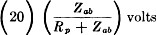
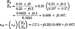
In order to find the voltage eg2 we must first find the voltage between the points A and B. The impedance Zab in series with the plate resistance Rp forms a voltage divider. Therefore, the voltage across Zab will be equal to
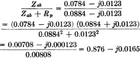
Rp is 10,000 ohms resistance or 0.01 + j0 megohms. Therefore, Zab + Rp = 0.0884 - j0.0123 megohms.
eab=(20) (0.876- j0.0165) =17.52- j0.33 volts.
Fig. 6 - Equivalent circuit of the resistance-coupled amplifier in Fig. 5 for low frequencies.
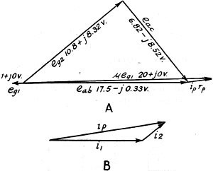
Fig. 7 - Vector diagrams useful in checking calculations. (A) shows the relative values of voltage in the circuit of Fig. 6, while (B) shows relative currents. The voltage eab is the sum of eg2 and the voltage drop across the coupling condenser since they are in series. Therefore, eg2 = (eab) (Rg/Z2)
The absolute value of this voltage is
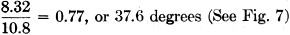
The overall amplification or ratio of voltage at grid No. 2 to that at grid No. 1 will then be 13.6, since one volt was assumed to be applied to grid No. 1. The voltage at grid No.2 will lead the voltage at plate No.1 by an angle whose tangent is
It is not necessary to find any phase angles to determine the voltage or current anywhere in the circuit. In fact, the relative phase of any voltage in the circuit can be found by graphical methods with sufficient accuracy for ordinary purposes. The fact that the voltages are expressed as complex quantities makes it easy to draw a scale diagram of the various voltages in the circuit. Such a diagram is useful for checking the accuracy of the calculations. A diagram of the voltages in this circuit is shown in Fig. 7, and a diagram of the relative currents is shown in Fig. 8. The values of alternating current in microamperes can be found by multiplying the admittance in micromhos by the applied e.m.f. of 20 volts (I = EY). The voltages and currents considered in this problem are, of course, only the alternating parts of the pulsating voltages and currents in the actual amplifier. The d.c. values have no other effect than to establish the values of Rp and μ and to determine the amplitude of voltage that can be applied before distortion begins. In practical work the performance of amplifiers is ordinarily computed by means of graphs or approximate formulas rather than such detailed calculations. The examples given above were used instead of the usual problems concerning miscellaneous collections of inductance and capacity because they are typical of the circuits actually found in radio equipment, and thus should indicate that the methods of calculations illustrated have practical applications. One desirable feature of using complex notation is that it eliminates the necessity for extracting square roots except for one such operation as the last step in the calculations, when the absolute value of current or voltage is desired, as is usually the case. A vector diagram of all the values in the problem should be drawn as a check on the calculations and to make sure that plus signs have not been slipped in where there should be minus signs or vice versa. Such errors are usually readily apparent as soon as construction of the diagram is attempted. The vector diagram need only be drawn roughly to scale, and may be in terms of voltages, currents, impedances or admittances, whichever is most convenient. * ·12 Griggs St.. Allston 34, Mass. 1 Noll, "Meet Mister j," QST, October, 1943, p. 21. 22 B is sometimes defined as - X / Z2, making Y = G + jB, This of course, is equivalent to the relation given above.
Posted September 28, 2019 |
|